Lesson 8 Space and time

Traditionally, space was not relevant in simulation modelling. Classical approaches of System Dynamics were based on highly aggregated entities that ignore local spatial variations. Simulation models were designed to unravel the behaviour of systems in terms of their temporal dynamics. It is only since bottom-up approaches like cellular automata and agent-based modelling have gained momentum, that the simulation modelling community takes strong interest also in the spatial domain.

On the other side, the GIScience community identified the integration of ‘time’ as one of the top research areas ahead. Although, the ideas of incorporating time into geographic frameworks date back to Thorsten Hägerstrand’s thoughts on “Time Geography” in the 1970ies. In Figure 8.1, there is a representation of a red, a green and a blue object that travel around a city (2D map at the bottom) over time (z-axis). The result is a three-dimensional path through space-time. However, the full integration of the spatial and the temporal domain still poses challenges with a lot of interesting research questions to be solved.

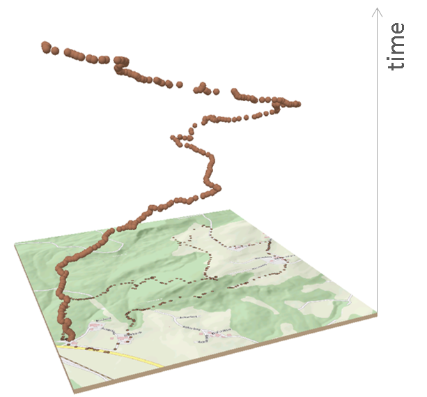
Figure 8.1: Space time paths visualise 2D movement over time, where the third dimension displays time.

In this lesson we will focus on spatial and temporal aspects, primarily from the perspective of the design of a simulation model and we will then briefly discuss integration of space and time to analyse emergent spatio-temporal patterns.

8.1 Space in simulation models

To design a simulation model, we need to think about how we want to model spatial features. On the one side this depends on the phenomenon, we are interested in. On the other side, aspects of performance need to be considered. As GIScientists, we are familiar with the concepts of how to represent geographic space in computer models. From the specific perspective of simulation modelling, four aspects are of particular importance:

• Spatial data models (vector, raster, graphs)
• Scale(s)
• Neighbourhood: Moore and more
• Boundaries: finite, infinite, toroidal

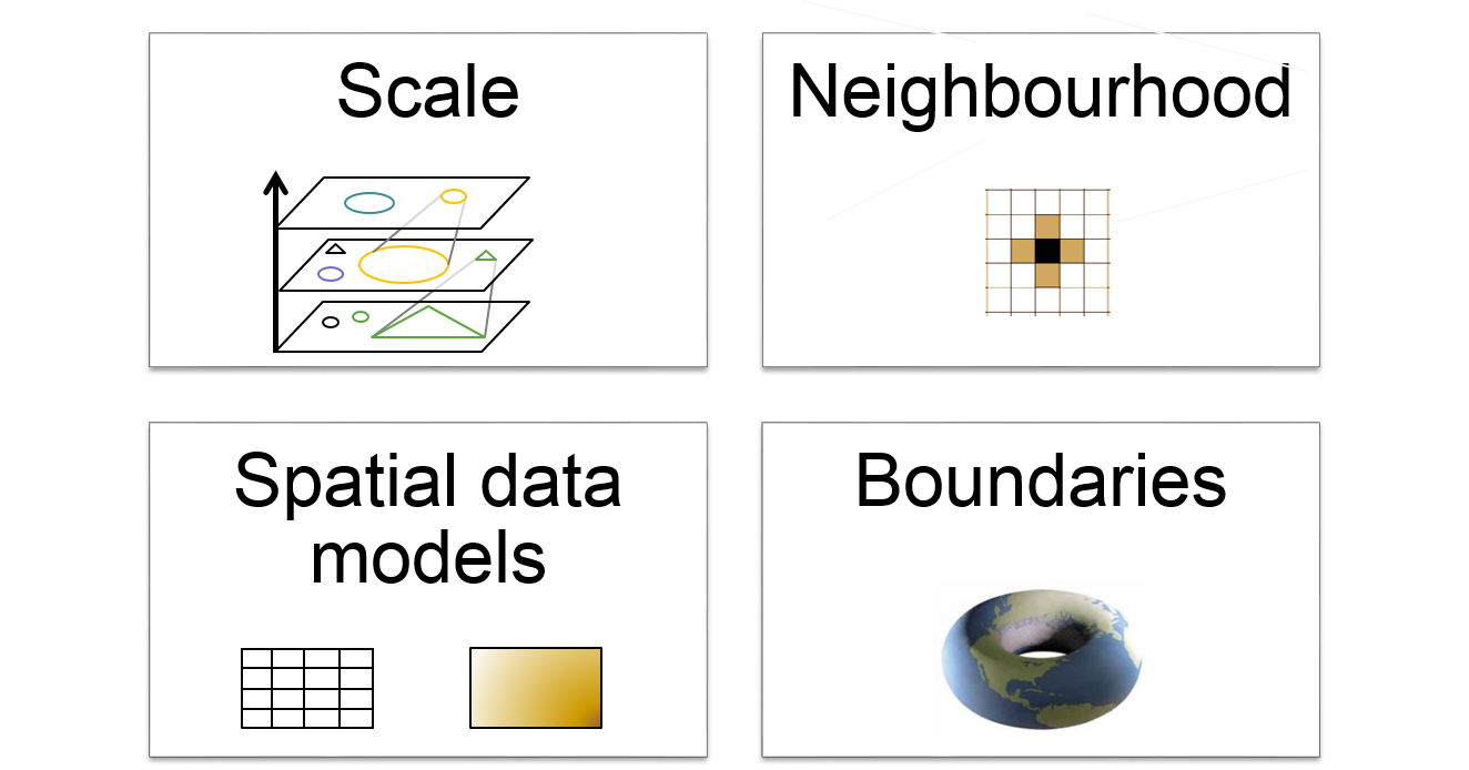
Figure 8.2: Important concepts of space in simulation modelling.

8.2 Spatial data models

An important decision during model design, is whether the phenomenon of interest is most adequately represented as vector, as raster, or as a graph.

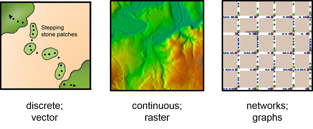
Figure 8.3: Space time paths visualise 2D movement over time, where the third dimension displays time.

The discrete-object view tends to work best in describing and representing biological organisms or human-made features such as buildings, vehicles, or fire hydrants. However, lastly it depends on the scale, whether a feature is discrete or not. For example, trees can be modelled as discrete entities or in aggregated form as a cell in a raster. If the entity is active on its own, an agent-based approach probably is best suited. Whereas, discrete non-living objects or land units can be adequately modelled in cellular automata. In contrast, the continuous-field view represents the variation of a variable over the Earth’s surface. There are no gaps in coverage, and there is exactly one value for each variable at each location. This view tends to work best in describing the variation of physical quantities, e.g. temperature or ground water level. Cellular automata are a typical modelling approach to deal with such phenomena. For processes that follow physical laws as fore example the diffusion of air pollutants in the atmosphere, a numerical model based on partial differential equations (PDEs) is likely to be a well fitting approach. Finally, graphs represent processes that operate on network structures, e.g. sewage canals or roads, but also flight paths of migratory birds, or connected habitat patches in a biotope network. As graphs represent topological relationships, these models can be more or less abstracted from geographic space. A common example for a graph-based simulation model are food web models. These models may, or may not be spatially explicit.

8.3 Spatial scale

Scale is another important decision that we need to take during model design. Often, this decision is taken without giving it explicit thought. In a simulation model, there are three scales that we can think about. The landscape ecologist Monica Turner defined these three scales as the scale of the modelled components, the level of focus and the scale of the environment that sets constraints to the model (M. G. Turner et al. 2001).

Figure 8.4: In simulation models we deal with (at least) three spatial scale levels. Source: Turner et al. (2001).

First, the scale of the components. It refers to the level of disaggregated stocks in spatial system dynamics models and to agents or cells in bottom-up simulation models. In cellular automata the scale at which one cell acts is given through the raster resolution and the neighbourhood on which it has immediate impact. In agent-based model this scale is defined by the agent’s potential range of movement and the maximum distance up to which it can sense its environment (the ‘vision’). Second, the scale of the phenomenon in which we are interested. It is the scale of the system, e.g. an ecosystem, a city or a sewage canal system. Third, the environment. This refers to everything ‘around’ the system of interest. As geographic systems are open systems, there are always flows of matter and / or energy into and out of the system. For example, in a population model young males may leave their home population and other animals may immigrate ‘from outside’.

8.3.1 Working with multiple scales

Traditionally, a simulation model focuses on one single scale. However, many processes happen at multiple scales simultaneously. For example, a predator-prey model can focus on the habitat range of one or several prey populations as well as on the predator habitat, where the size of habitats may differ by an order of magnitude. The interaction between scales can be represented with nested models. Such models need to be designed and analysed carefully in order to provide a sound ‘translation’ between scales and to avoid related fallacies:

• The ecological fallacy describes the inappropriate use of macro-level data to make inferences at an individual level. For example, if the an average success rate of a predator to kill a prey is one prey per day, this does not imply that the majority of predators succeed to have daily kills. The first state variable describes a mean value for the population, whereas the latter refers to the median. This problem of down-scaling was first described by Robinson (1950).
• The individualistic (atomic) fallacy describes the inappropriate use of individual-level data without considering their wider (spatial) context. This problem of up-scaling refers to the wrong assumption that only individual-level attributes can explain individual behaviour. For example age and gender alone does not suffice to explain the migration behaviour of a dolphin. The context of the school of dolphins in which it swims is also important.
• Finally, the cross-level fallacy describes the inappropriate use of data from one part of the system to make inferences about another part at the same scale. This is a problem of spatial extrapolation: a simulation model that was successfully validated for one study area is not necessarily valid outside this area.

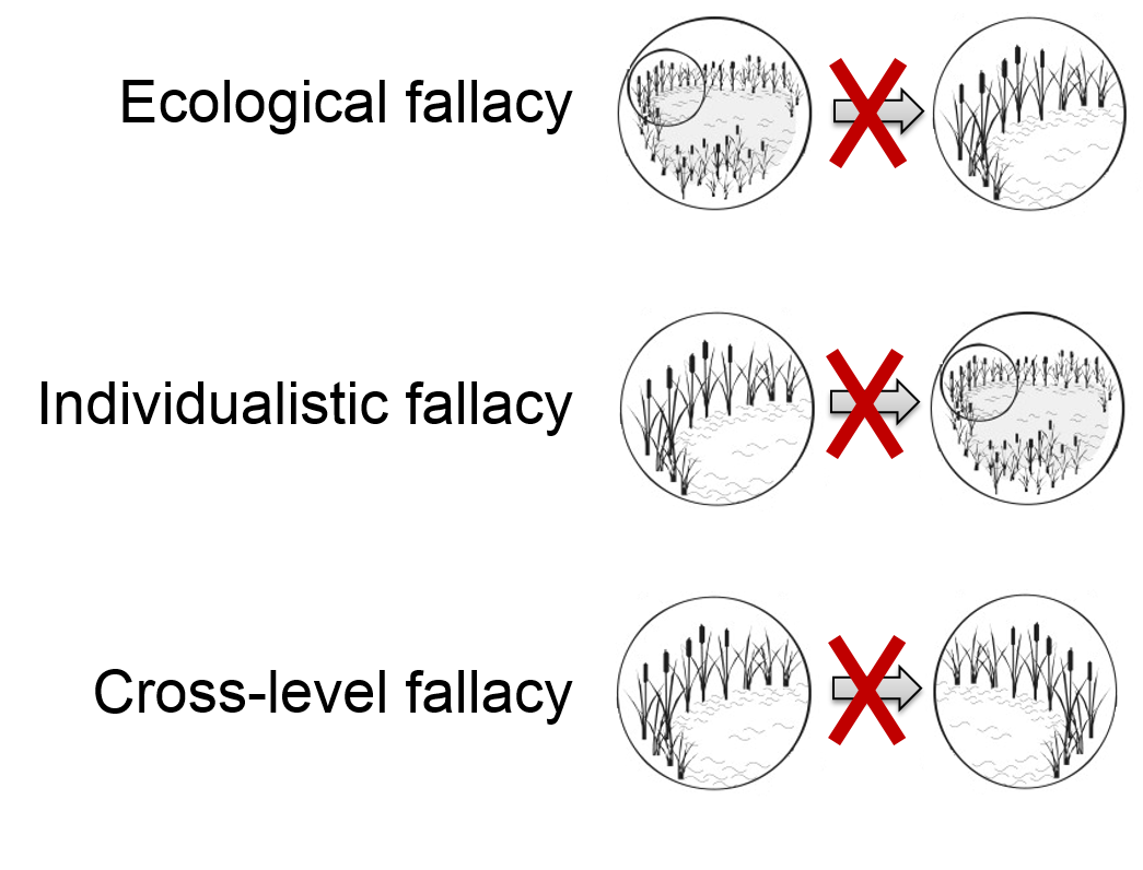
Figure 8.5: Translating between scales can cause severe inference problems (fallacies).

8.3.2 Fractal scales

Fractal scales assume self-similarity across multiple scales. Fractal patterns and processes are thus scale invariant and it is valid to infer from one scale to another, i.e. to up- and downscale. Natural phenomena are hardly ever fully fractal, but rather have fractal features. Prominent examples are frost crystals, fern leaves, erosion patterns, shore lines and mountain landscapes. The computer game and movie industry has taken advantage of this geometric property of landscapes in order to generate artificial sceneries that look realistic. The Star Trek movie “The Wrath of Khan” in 1982 was the first movie to use a fractal generated artificial landscape.

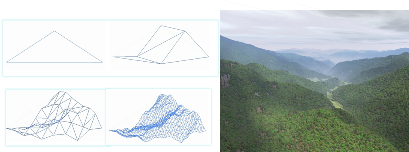
Figure 8.6: Fractal landscapes: the design of a synthetic landscape with a stochastic self-similarity that mimics natural terrain. The image on the right is a computer-generated fractal landscape rendered by Gary R. Huber with Visual Nature Studio, 3D Nature, LLC.

The concept of fractals was introduced by Mandelbrot (1977) and later has been adopted for landscape analysis (e.g. M. G. Turner et al. 2001). The degree of ‘fractalness’ is expressed by the fractal dimension (D), which describes the complexity of a polygon by relating the perimeter (P) of a pattern to its area (A) by \(P\sim A^D\). For simple Euclidean shapes (e.g., circles and rectangles), \(P\sim\sqrt(A)\) and D = 1, the dimension of a line. As the polygons become more complex, the perimeter becomes increasingly plane-filling and \(P\sim A\) with \(D\to 2\). In simulation modelling, fractal artificial landscapes can be used as ‘neutral landscape models’ against which landscape patterns can be compared (Gardner et al. 1987). Fractal landscapes in landscape analysis are thus the null hypothesis against which real or simulated landscapes can be compared - just like ‘complete spatial randomness’ patterns in point pattern analysis.

8.4 Neighbourhood

Local interaction processes in bottom-up simulation models take place in a certain neighbourhood. The shape of this neighbourhood greatly influences the shape of emerging patterns. In a cellular automaton, the geometry of a neighbourhood is given by the type of neighbourhood and the type of tesselation of the underlying space. Previously in this module, we have discussed various types of neighbourhood, including von Neumann, Moore, directional or stochastic neighbourhoods. These neighbourhood types can differ significantly when applied to different underlying grid structures.

In the top row of Figure 8.7 there is a Moore neighbourhood as it manifests itself on various tesselations or in continuous, Euclidean space. The same principles are also true in network geometries, where line segments can be split differently, e.g. at equal distances, at intersections, or related to attribute changes.

In the bottom row there are the respective isoclines of distance. The rectangular grid exhibits a bias in the distance depending on the direction, which leads to artifacts in emerging patterns: adding a buffer to a centre cell results in a square instead of a circle. In contrast, Voronoi tesselation does not lead to biased patterns. Although Voronoi grids exhibit irregular isoclines at near distances, these Irregularities even out at farther distances. The most common grid structure – the raster of rectangular cells – is also the most problematic. One way to overcome unwanted artifacts is to include stochastic neighbourhoods that are weighted by the inverse of their Euclidean distance, where all von Neumann neighbours have a weight of w=1 and the diagonal Moore neighbours have a weight of \(w = \frac{1} {\sqrt(2)} = 0.7071\) .

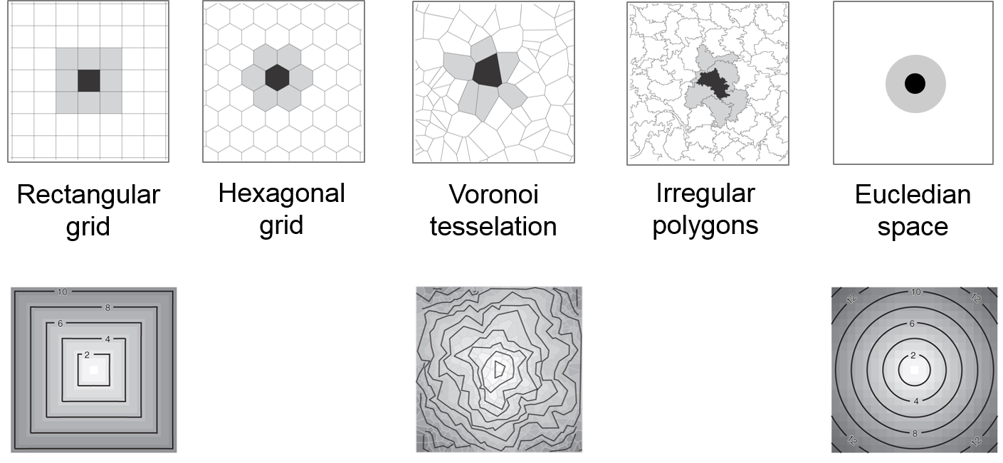
Figure 8.7: The same neighbourhood implemented in different grid structures.

8.5 Boundaries

Figure 8.8: ‘Here be dragons’” – in ancient maps, the end of the world was symbolised with scary-looking dragons.

In simulation modelling there are several ways to handle these dangerous fields:

1. The world ‘ends’ at the boundary
   This is a pragmatic approach that is usually applied for real-world study areas. The open question is how to simulate local neighbourhoods beyond the borders. In cellular automata, the rows at the edge need to adapt their neighbourhood rules to the reduced number of actual neighbours. Agent-based models with moving agents often have a ‘bouncing’ algorithm, where the agent turns by 180° or where it bounces like a ball on a snooker board. Alternatively, the model can be designed to allow agent to leave the scene and in turn allow other agents to enter.
2. The world wraps
   Wrapping worlds are often used in homogeneous (artificial) landscapes: an agent that leaves the scene on the left re-enters at the right side. It is a common approach in abstract, theoretic models. This never-ending concept of space is called toroidal (‘doughnut-like’) space.
3. Infinite space
   Simulation models that operate in infinite space extend themselves as an agent approaches the boundaries. Clearly, this approach can quickly get computational extensive. However, it might be adequate, if the model follows a single agent, or a cluster of agents, that moves over long distances.

8.6 Time in simulation models

Time is sometimes handled as ‘just another dimension’. For many cases this pragmatic view is a useful way to think about time. Analogous to the spatial dimensions, the choice of scale and data model types are of decisive importance. However, time has some peculiarities that we need to think about and explicitly address during model design. Unlike space, time has a direction and it is only one-dimensional. This makes the adequate order of update routines and scheduling of processes an important factor in the model design process. Finally, time often exhibits a cyclic nature that is given by the day / night rhythm and seasonal changes. Therefore, the state of the system a year ago may be more relevant in predicting the upcoming change, than the state two months ago.

There are four aspects in the representation of time that are important from a modelling perspective:

• Temporal data models
• Temporal scale
• Update routines (synchronous / asynchronous)
• Scheduling (Process timing)

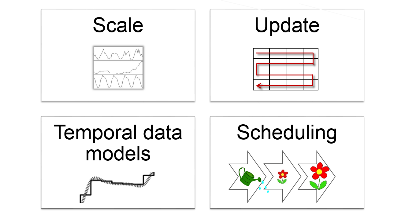
Figure 8.9: Temporal concepts in simulation modelling

8.7 Temporal data models

Time is a continuous phenomenon. Nevertheless, to represent time in a digital model, time needs to be discretised. Strictly speaking, even equation-based simulation models need to be discretised for computation. However, the actual parameter value can be computed for any point in time and we can think of these models as continuous models in the context of simulation modelling. In rule-based models (cellular automata and agent-based models) time is conceptualised in discrete time steps.

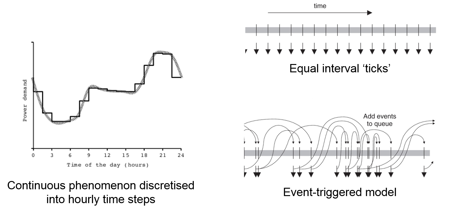
Figure 8.10: Temporal concepts in simulation modelling

The choice of how to represent time in a simulation model depends on the modelled phenomena:

• Continuous temporal phenomena describe an ongoing process, like temperature change or tree growth. System dynamics are the classical approach to model such phenomena. If we have a strong interest in how the process operates in space, a cellular automaton approach is more adequate. In this case, the continuous process needs to be broken down into time steps that are small enough to adequately represent the dynamic behaviour of the modelled process.
• Discrete temporal phenomena are termed ‘events’. Events can happen regularly, e.g. each morning the sun rises and thus triggers multiple processes: flowers open, birds become active, etc. Such events are well represented in classical cellular automata and agent-based models, where time steps usually are assumed to be regular. However, events are often irregularly paced, e.g. natural catastrophes. Such irregularity of events can be addressed by a fine resolution of discrete steps, where there is only a certain probability that an event happens. For systems that are strongly governed by irregular events, it is probably more adequate to apply an event-based approach, where events trigger the placement of later events in a queue.

8.8 Temporal scales

Many aspects that we have discussed for spatial scales are also valid for the temporal scale. In the model design phase, we explicitly consider scale by defining resolution through the duration of a time step and extent through the duration of a simulation run. Further, we can transfer the landscape ecological concept of the three levels of spatial scale to the temporal domain:

• The temporal scale of system components is governed by the granularity of agent processes. An agent processes can be limited to one time step only, if the change simply depends on the current state of the system, e.g. in Markov chain models. More complex models conceptualise agents to have a memory and thus consider processes with a – sometimes considerably – ‘extended temporal neighbourhood’.
• The focus scale relates to time frames of emergent phenomena at system level. Simulation runs typically are laid out to meet expected time frames of emergent phenomena.
• Finally, ‘environmental’ constraints are set by a system’s history. Often these constraints are acquired empirically, e.g. land cover state at simulation start can be derived from an orthophoto. Frequently, simulations need a ‘start-up phase’ to avoid artifacts in the dynamics of emergent process that are due to ‘boundary effects’, for example while agents build up their memories.

A highly frequent aspect in the temporal domain is self-similarity. The cyclic nature of time, which is rooted for example in day-night oscillations or seasonal changes, leads to strongly fractal properties of temporal phenomena. In temporal data analysis, we can utilise this property of time to decompose spatio-temporal patterns into multiple scales (see Figure 8.11).

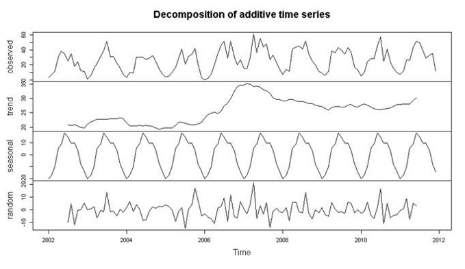
Figure 8.11: Decomposition of bicycle accidents in the city of Salzburg over 12 years (top row) into two temporal scales: the 12-year trend (2nd row) and a repetitive seasonal pattern (3rd row). The bottom row shows a random noise as remainder.

8.9 Scheduling

Scheduling refers to the order of processes through which an agent or cellular automaton iterates at each time step. For some processes there is a clear, sequential order, but in many cases real world processes occur concurrently. However, in a computer model it is only possible to run one process at any time and we thus need to decide in which order processes actually are being executed. This execution order can strongly effect simulation results. For example, the amount of new seedlings depends on the order of the processes ‘old-trees-die’ and ‘trees-disperse’. There are several strategies to overcome such bias:

• we can define a random order of concurrent processes so that potential biases equal out over time.
• If several processes have different duration, we can design a nested schedule: e.g. a daily process will be executed each time step, whereas a weekly processes only each 7th time step.
• Further, time steps can be designed to have different duration, e.g. hourly during the day and three-hourly over night.

To assess in which way and how much a changed schedule affects the outcome of a model, we can reorganise the execution order of concurrent processes and compare the results. This can be an important aspect in the model validation strategy.

8.10 Updating

Updating refers to the spatial order in which a process implements a change of state in the system components. There can be significantly different outcomes, if all cells (or agents) are updated at the same time, or one cell (agent) after the other.

• The default case is a synchronous update, in which all cells are updated at the same time: first, the future states are computed for each cell and then these changes are executed.
• In some cases an asynchronous update is more adequate. In this case, the future state for the first cell is computed and immediately executed, then for the second cell and so forth, until the end. The future state of a cell thus depends on neighbours that might have, or have not already been updated. The update sequence usually is random, but it can also be handled row by row in a fixed queue – although this latter case is unlikely for real-world processes. It is more likely, that the update sequence is governed by an attribute. For example, the wealthier a household is, the earlier it can choose a free flat to move to. This way, a model represents the greater choice that rich people have when looking for a flat.

Simulation outcomes may differ significantly between updating algorithms. Interestingly, also the modelled process itself greatly influences its sensitivity to update routines. In Figure 8.12, the update starts from a random pattern (top) according to the Majority rule (left) or the Game of Life rule (right). For the Majority rule, the update procedures do not differ much, except for the asynchronous, fixed queue update. Here, patches propagate over the grid and form larger patterns. In contrast, the Game of Life rule results in a tremendous difference between synchronous and asynchronous update rules.

Figure 8.12: The effect of different updating orders in a cellular automaton. Source: (O’Sullivan and Perry 2013)

8.10.1 Asynchronous update

Asynchronous update algorithms are well suited to represent different process rates. Let’s consider two animals, which are both feeding on nuts: mice and squirrels. Whereas a mouse only eats on average 5 nuts a day, a squirrel usually eats about 50 nuts. The feeding processes thus are concurrent, but happen at different rates. We could now schedule first the squirrels as they are obviously quicker then mice. However, in case of nut shortages mice are likely to starve, which is not realistic. Further, if mice and squirrels have different spatial search strategies, the spatial distribution of remaining nuts will be different.

Figure 8.13: Mice and squirrels feed at different rates

To overcome this problem, we apply an asynchronous update strategy:

First, we assign the probabilities of mice and squirrels to find and eat a nut by dividing the respective processes rates by the total rate: \(p_{i}=\frac{r_{i}}{r_{i+j}}\). In our case the squirrel eats 50 nuts per day and the mouse feeds only 5 nuts per day. So the update probability of a mouse is p = 0.1 and of a squirrel p = 0.9. Now, we define one day with 50 time steps. At each time step either the mice (10%) or the squirrels (90%) can choose and eat a nut.

8.11 Summary

As GIScientists we are used to think about peculiarities of the spatial dimension. We know about continuous and discrete spatial representations; about scale and the problems of combining different scales; and about topological neighbourhood conceptions and how they vary depending on the underlying discretisation of space. Characteristics of the temporal domain may be less familiar to us. Some concepts like ‘scale’ and related issues can be easily transferred. Other issues relate to the directionality of time. When we work with computers we only can represent one process a time (unless we work with parallelisation, which opens up a new level of complexity). Therefore, we cannot represent concurrent events and need to define sequences of update routines. The nature of these sequences can make huge differences. Equally we need to think about scheduling of concurrent processes within a time step, e.g. continuous processes (tree growth) vs. dispersal events.

References

Mandelbrot, Benoit. 1977. Fractals. Freeman San Francisco.

O’Sullivan, David, and George LW Perry. 2013. Spatial Simulation: Exploring Pattern and Process. Book. John Wiley & Sons.

Robinson, William S. 1950. “Ecological Correlations and the Behavior of Individuals.” American Sociological Review 15 (3): 351–57.

Turner, Monica G, Robert H Gardner, Robert V O’neill, Robert H Gardner, and Robert V O’Neill. 2001. Landscape Ecology in Theory and Practice. Vol. 401. Springer.