Lesson 6 Cellular Automata
This lesson introduces into the principles of designing cellular automata (CA) models by relating to the three components of a system’s model: purpose, elements and relations. CAs are a method for spatially-explicit, bottom-up modelling of dynamic environments. In its early days this approach triggered great interest in the “life-like” behaviour that emerged from these computer models. Conway’s “Game of Life” fuelled the discussion on intelligent or even human-like machines. Indeed, artificial intelligence technology has evolved a lot since then, and whether or not machines can potentially be “intelligent” is one of the hot questions in today’s philosophy of science. Until today, the undebated strength of CA is their ability to represent the underlying mechanism of how local processes operate and thus CAs have the potential to demonstrate, how spatial patterns are produced and serve as virtual labs for scenario analyses.
Upon completion of this lesson, you should be able to…
- decide whether a specific system is adequate to be modelled with Cellular Automata based on its elements, interconnections and the purpose of the model
- how CA models are implemented, and
- list typical problems that are studied with the CA approach.
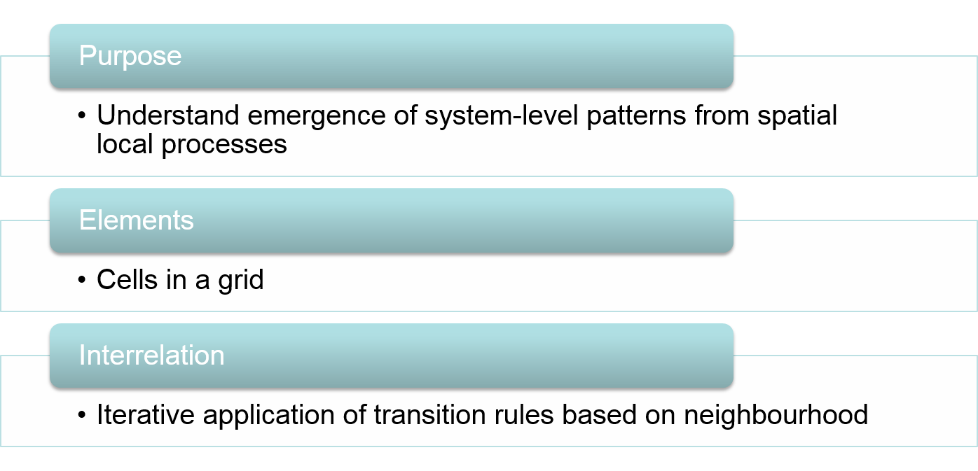
Figure 6.1: Conceptual view on modelling systems with the Cellular Automata approach
6.1 Purpose
The purpose of cellular automata is to simulate the dynamic evolution of extended spatial phenomena at system-level emerging from local processes. Whereby local processes are represented mechanistically by transition rules for the state of individual cells that depend on their own state and the state of cells in their local neighbourhood.
Cellular automata implement Tobler’s First Law into simulation modelling. In a nutshell: the status of a cell in the next time step results from the current status of itself and its neighbours. The state transition of a cell is evaluated iteratively in discrete time steps. Such iterative repetition of local (and simple) transition rules simulate the emergence of system level patterns over time. All we need to define is the relevant neighbourhood and the rules of change.
The credit for the first conceptual idea for cellular automata is given to the Austro-Hungarian mathematician John von Neumann. Von Neumann aimed to simulate self-reproducing, self-organised ‘living’ patterns. When John Conway implemented this idea in the 1960ies with extremely simple rules of cells that can switch between two states according to the state of their neighbours, the “Game of Life” was born (Gardner 1970). At that time, cellular automata seemed to be nothing more than a game. However, the result of this seemingly simplistic approach was a variety of surprisingly complex behaviour. This created a lasting enthusiasm in many research communities. Finally, Stephen Wolfram (2002) developed an entire body of theory around cellular automata.
A plethora of cellular automaton models have been developed to solve theoretic and increasingly also applied problems of spatial processes. Often, cellular automata models are used in combination with other techniques mostly agent-based models, or probabilistic modelling techniques such as neural networks or Markov chains. Further, cellular automata can also be used as stepwise (discrete) approximation models to solve partial differential equations.
6.2 Elements: cells
The basic modelling unit of CA models are the cells in a grid, where each cell has a certain state. In its simplest type the state is binary, such that a cell’s value can only switch between two states, e.g. “on or off”, or “black or white”. However, it is also possible that a cell can take several possible states at any level of measurement from nominal to metric, e.g. land-use classes, land capability class, temperature, or biomass.
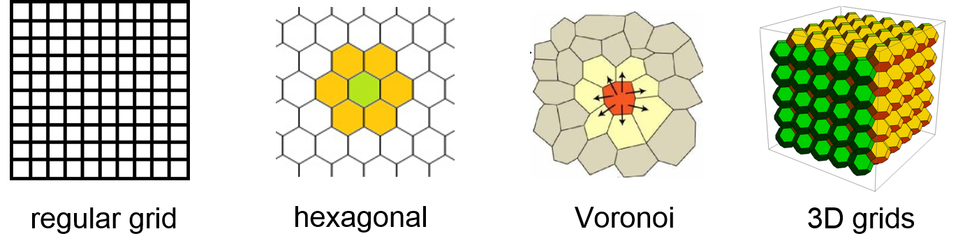
Figure 6.2: The basic elements of cellular automata are cells in a grid.
Some models are abstract, such that a grid cell does not refer to a certain location in the real-world. For empirical models that take ‘real-world’ data as an input, one cell represents a certain extent e.g. one square meter in a specific study area. Such models can also be validated with empirical observations, e.g. measurements from a sensor network or remote sensing data. Typical CAs are implemented in a rectangular grid. However, it is equally possible to model hexagonal cells or even irregular Voronoi polygons.
6.3 Relation: transition rules
6.3.1 Neighbourhood
Where happens what? These two “w” questions need to be answered to be able to model how a system changes from one time step to the other. The ‘where’ is pre-structured by the chosen grid structure and defined by the neighbourhood that needs to be considered (Figure 6.3). In a rectangular grid, there are two possible neighbourhood concepts. The ‘von Neumann’ neighbourhood considers only the four directly adjacent cells, whereas the ‘Moore’ neighbourhood includes also the four edges and thus considers eight cells. For processes that operate over larger distances, a larger neighbourhood must be defined. Finally, a process can have a directional component, as for example wind that drives wildfire into a certain direction. In principle, any arrangement of cells can be defined as neighbourhood, but they are all composed of the four above aspects: grid structure, neighbourhood type, distance and direction.
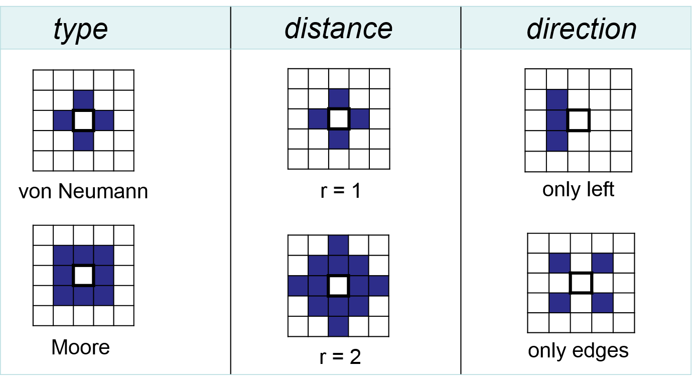
Figure 6.3: The neighbourhood defines the spatial structure of how cells are connected in a CA model.
In Figure 6.4 there are the respective isoclines of distance of the same circular neighbourhood, mapped to different grid structures. The rectangular grid exhibits a bias in the distance depending on the direction, which leads to artifacts in emerging patterns: adding a buffer to a centre cell results in a square instead of a circle. In contrast, Voronoi tesselation does not lead to biased patterns. Although Voronoi grids exhibit irregular isoclines at near distances, these irregularities even out at farther distances. The most common grid structure – the raster of rectangular cells – is also the most problematic.
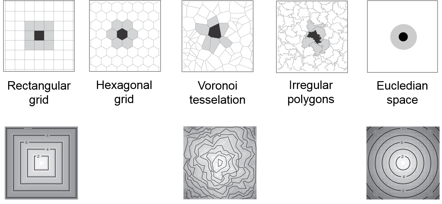
Figure 6.4: The same circular neighbourhood concept, implemented in different grid structures.
Exercise: Neighbourhood of a process
Explore the model in Figure 6.5. Open the NetLogo Code tab and check lines 30 to 40: which cells are considered as neighbourhoods to represent the three wind directions?
Figure 6.5: Explore, how different local process neighbourhoods impact the system-level outcome, NetLogo Web
6.3.2 Transition rules
Transition rules are the true process engines. They govern the actual nature of change, as they define the ‘what’ in answer to our question: where happens what?
Transition rules specify how cells change their state from one time step to the next. The specified set of rules equally applies to each cell in the grid and it is applied to all cells simultaneously. In classical CAs, cells do not have a memory, so that only the state of the previous time step is considered. The subsequent state of a cell is determined by the state of the cell itself and the state of its neighbours. There can be an arbitrary number of rules, but the rule set needs to consider all possible combinations of situations that can occur in the neighbourhood of a cell.
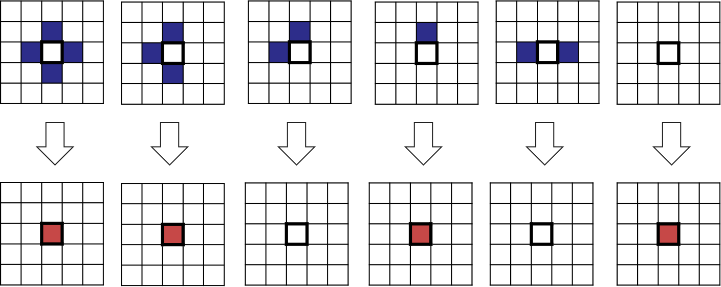
Figure 6.6: Transition rules define the local interaction between cells in a neighbourhood.
Deterministic CA’s specify transition rules exactly with help of ‘if-else’ statements. However, it is also possible to add stochasticity by introducing probabilities of change. The first case applies mainly to abstract models that are based on theoretic considerations, whereas stochastic processes that are rooted in empirical relationships usually result in more realistic appearance.
6.4 Conway’s Game of Life
Conway’s Game of Life provides us with an excellent example of studying a cellular automaton ‘at work’. It considered an eight-cell Moore neighbourhood and has a set of four simple transition rules:
At each time step any living cell
- with 0 – 1 neighbours dies (‘rule of loneliness’)
- with 2 – 3 neighbours stays alive (‘survival rule’)
- with 4 – 8 neighbours dies (‘rule of over-crowdedness’),
any dead cell
- with exactly three living neighbours comes to life (‘three parents rule’).
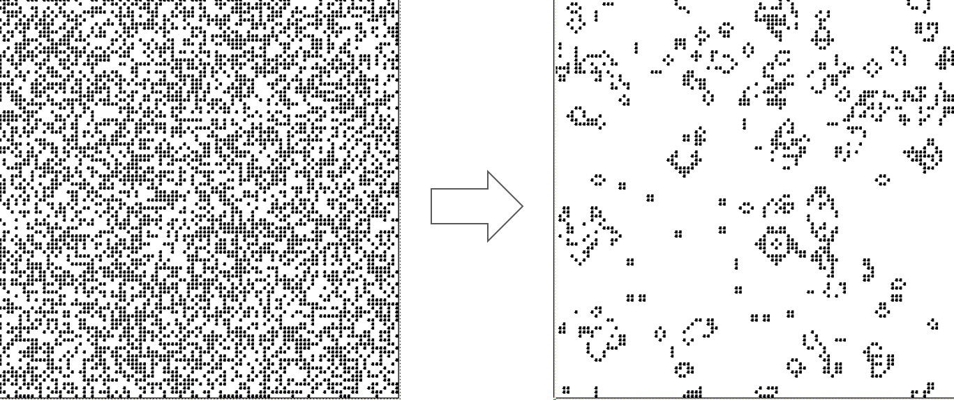
Figure 6.7: The Game of Life in action: from a random configuration of dead and alive pixels, a number of life-like structures emerge.
In the Game of Life, only the number of neighbouring cells matters, their spatial distribution is irrelevant.
What are the results of the Game of Life - which spatio-temporal patterns emerge? As the Game of Life is deterministic, a certain initial condition always results in the same pattern. However, the results can be quite striking and they are by no means intuitively predictable. The following Figures 6.8, 6.9 and 6.10 show three typical emergent Game-of-Life patterns:
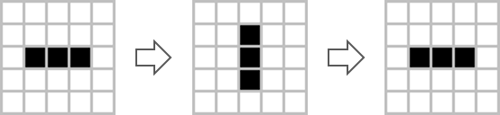
Figure 6.8: The ‘blinker’ that oscillates between two states.
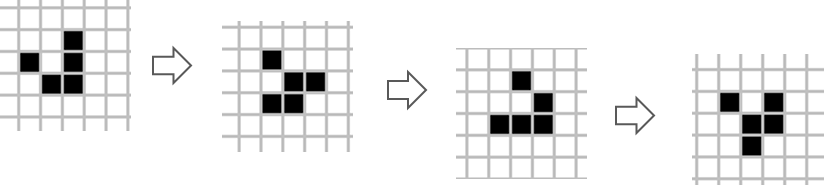
Figure 6.9: The ‘glider’ that moves over the grid.
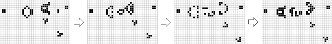
Figure 6.10: The ‘breeder’ constantly creates moving gliders as the two ‘parents’ meet.
Other patterns die out, transform into a stationary pattern, or generate large, irregular patterns that take >1000 steps until they become stationary or periodic. As researchers discovered the properties of these structures, they were enthusiastic about the complex, life-like behaviour that develops from a set of such simple rules. The notion of artificial life was formulated and expectations were flying high of what is there to come.
Exercise: Game of Life
Here it is: The model in Figure 6.11 implements the Game of Life model in NetLogo. Draw a blinker and see, whether it works!
Figure 6.11: The Game of Life model, NetLogo Web
6.5 Self-similarity
Besides the emergence of life-like patterns there is another striking property of cellular automata: self-similarity. Self-similar patterns show the same or similar shapes at multiple scales. A self-similar object thus is similar or approximately similar to a part of itself. This is a quite common pattern in nature. Figure 6.12 shows self-similarity for two very distinct natural objects: the tips of the maple leaf and the undulating pattern of the northern shoreline of the African continent repeat themselves at multiple scales. The phenomenon of self-similarity can also be observed in mountain landscapes, fluvial erosion, or the growth of cities and urban sprawl.
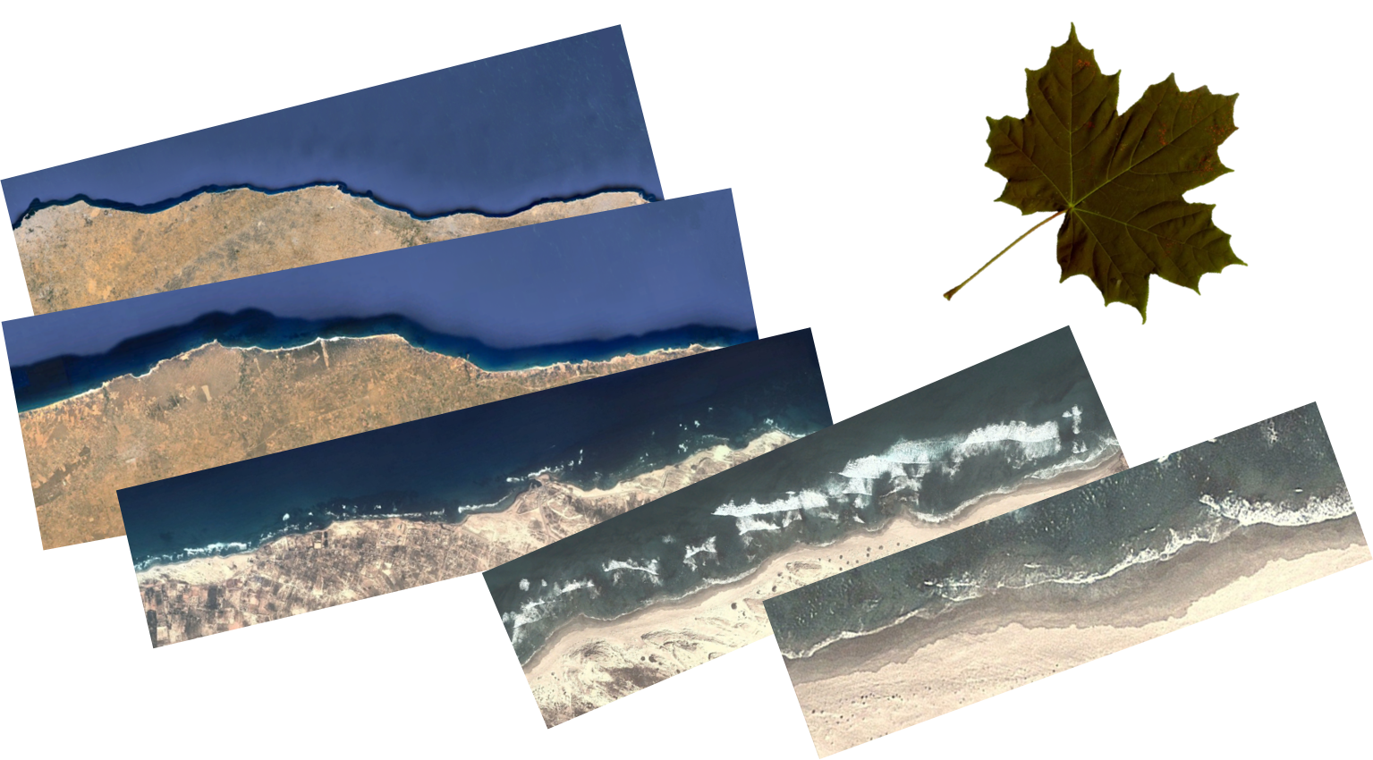
Figure 6.12: The shore of the northern African shoreline and the maple leaf are examples of self-similar structures in nature.
Cellular automata help us to understand the process that is responsible to create self-similar patterns. Consider a CA that models water run-off from a hill. The water will run down the hillslope and bit by bit erode the flow channel. The simulation outcome in Figure 6.13 shows the characteristic self-similar pattern of fluvial erosion.
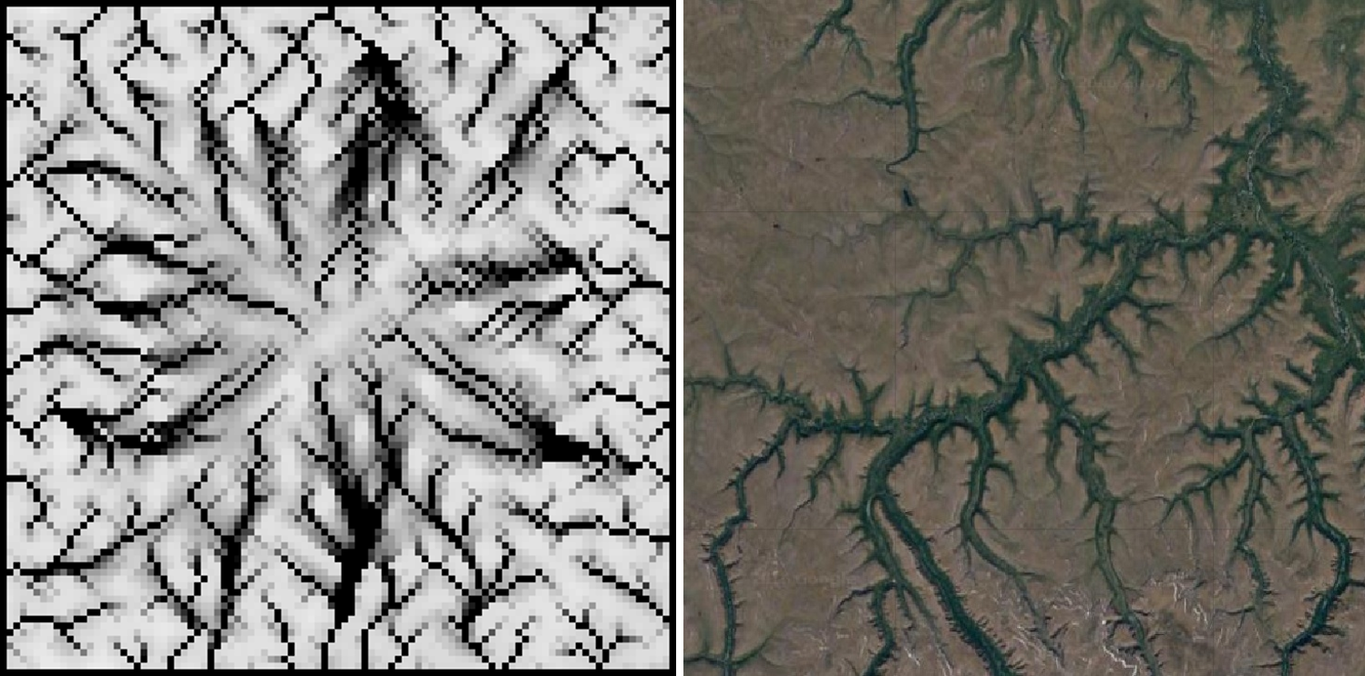
Figure 6.13: Fluvial erosion generates the dendritic self-similar structures of river networks. Left: erosion patterns generated by a CA model, right: a satellite image of a river
Cellular automata thus can help to explain, how self-similar landscape forms may have evolved. Further, we can use self-similar cellular automata to generate realistic ‘artificial’ landscapes, e.g. for computer game landscapes – or in our case for theory-based simulation experiments.
6.6 Geographic CA’s
Having discussed two of the main emergent properties of CA’s, i.e. the generation of life-like structures and self-similarity, we now will stepwise move from abstract grids with a limited number of cells to the application of CA models to real-world, geographic environments. The abundance of remotely sensed data opens the possibility to run simulations of realistic landscapes.
Let’s consider local settling processes, where one settler builds his house next to an existing house, while he tries to have as much green space around as possible. This is the typical situation that leads to urban sprawl.
A small caveat at this place: increased realism not always is what we are striving for in simulation modelling. Too much detail may obscure cause-effect relationships between individual behaviour and emergent system-level patterns. To better interpret the behaviour of complex systems, it often helps to understand the behaviour of simple models.
6.6.1 Deterministic CA
Translated into CA transition rules, the model will simulate a pattern that grows from the centre into 2D space. Each time we start the model, the result will look exactly the same. However, the result looks quite artificial, as you can see in Figure 6.14.
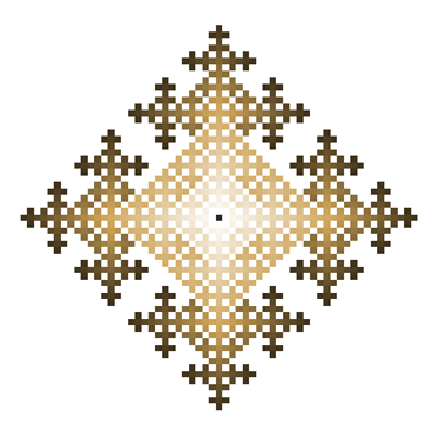
Figure 6.14: Deterministic CA: a cellular automaton the grows according to strict, deterministic rules will always result in the same pattern
Exercise: deterministic CA
Work yourself through the code of a the deterministic CA that grows according to a Moore neighbourhood. Note, how a variable of type “myCA” can be declared to hold a specific cell. And also find an example of how to use the pseudo-variable each.
See the code of a deterministic CA, growing in a Moore neighbourhood.
/**
* Name: Ex L5a - deterministicCA
* Author: WALLENTIN, Gudrun
* Description: Exercise of the UNIGIS Salzburg optional module
* deterministic CA
*/

model ExL5a_deterministicCA

global  {
  myCA centre_cell <- myCA[49,49];

    init {
        ask centre_cell{
            switch <- true;
            color <- #red;
        }
    }

    reflex switch{
        //only consider cells that are already switched
        ask myCA where (each.switch = true){
            ask neighbors {
                switch <- true;
                color <- #red;
            }
        }
    }
}

//The cellular automaton
grid myCA width:100 height:100 neighbors:8 {
    bool switch;
}

//Simulation
experiment simulation type:gui {
    output {
        display map type: opengl{
            grid myCA;
        }
    }
}
Take a moment to think about what would happen, if we allowed the deterministic rules of the model in the figure above to be random in 10% of cases? How will the resulting pattern look like?
6.6.2 Stochastic CA
A model that follows a set of rules with some random component is called a stochastic model. Figure 6.15) is a good example of a stochastic CA that generally follows the same rules as the model in 6.14).
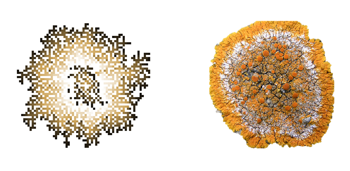
Figure 6.15: Stochastic CA: allowing only 10% randomness has a significant impact on the resulting CA pattern (left) which resembles much better organic, living structures like a lichen (right).
The emerging pattern is slightly different each time we run the model. More importantly, the pattern is quite different from the strongly geometric outcome of the deterministic model with the same rules. A small share of stochasticity overcomes also the problem with the geometry of CA’s on rectangular rasters, in which growth processes also result into a quadratic instead of a circular shape.
Now, imagine what will happen, if we apply the same, stochastic growth rules to geographic space, where transition rules (building of new houses) are effected by geographic features (e.g. streets or rivers)?
There is only a little code chunk that has to be added in order to convert a deterministic to a stochastic CA. Go ahead and add a where facet to the ask neighbors loop:
    ask neighbors where (rnd(1.0) < 0.2){
        switch <- true;
        color <- #red;
    }
Exercise: Display information in a chart
To track the state of a simulation quantitatively, we can add plots to model that display the information in real-time as the simulation runs. So, let’s take the model of the stochastic CA and add a time-series chart that plots the number of switched cells over time. As we want to display information about the amount of urban cells in the grid, the pseudo-variable each is needed to evaluate each value for the variable of interest in the grid.
display switched_cells type: java2D {
  // plot amount of cells which have been developed
  chart "myChart" type:series {
      data "Nb of city grid cells" value: myCA count (each.switch = true);
  }
}
If you want to display information of some statistics on the raster, e.g. the mean or the sum of all urban cells in the grid, you can make use of the statement collect. This statements collects the values of a variable of all grid cells into a temporary list on which you can execute your stats. The code below plots the average grid_cell score of switched cells.
However, when you run the code, you will realise that it works technically, but the value will remain zero.
display distance type: java2D {
  // plot the average score of cells
    chart "Suitability" type: series {
      data "Mean distance" color: #red value: mean(myCA where(each.switch = true) collect each.grid_value);
  }
}
To make the chart work, you need to compute the distance to the centre for each cell to the centre and write it into the grid_value variable. The most efficient way to do that is to compute the distances once, at the beginning for all cells. The command in the chart where(each.switch = true) filters only the relevant cells that have switched to city cells and computes the mean distance for this subset of cells.
6.6.3 Constrained CA
In a constrained CA, transition rules are only applied, IF a local condition is true. The constraint in the below example (see Figure 6.16) is the street network along which new houses are built.
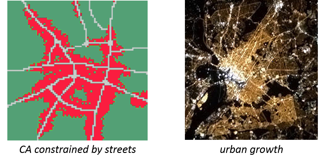
Figure 6.16: Constrained CA: the growth process is here constrained to the vicinity of a street (left). The resulting structure is similar to the structure of a real city (right)
The similarity between the CA model and the city structure is not just a random coincidence. Cellular automaton models aim to represent real local processes. If they do so successfully, the emerging pattern in the model matches with our real-world observations.
Exercise: Conditional structure
To implement a constrained CA, you need to execute the switch only IF a certain condition is true. For example, the cell only switches, if it is close to a street. The example below combines the constraint with a stochastic approach: the switch probability is higher, if there is a street nearby. Can you code that? Let the street geometry be the following set of points in a 100 by 100 cell grid and give it a try!
street_geom <- line([{0,0},{5,10},{10,20},{20,50},{30,70},{35,90},{40,100}]) + line([{50,0},{50,25},{55,73},{45,88},{40,100}]) + line([{0,45},{25,65},{45,50},{72,53},{100,35}]);See an example solution for the constrained (and stochastic) CA.
/**
* Name: Ex L5c - constrainedCA
* Author: WALLENTIN, Gudrun
* Description: Exercise of the UNIGIS Salzburg optional module
* constrained CA
*/

model ExL5c_constrainedCA

global  {
    geometry street_geom;

    init {
        ask myCA[49,49]{
            switch <- true;
            color <- #red;
        }
        street_geom <- line([{0,0},{5,10},{10,20},{20,50},{30,70},{35,90},{40,100}]) + line([{50,0},{50,25},{55,73},{45,88},{40,100}]) + line([{0,45},{25,65},{45,50},{72,53},{100,35}]);
    }

    reflex switch_{
        //only consider cells that are already switched
        ask myCA where (each.switch = true){
            //the chance to switch is higher, if close to street
            ask neighbors {
                //ask the neighbours of switched cells that are close to streets to switch with a 70% chance
                if (self distance_to street_geom < 5 and flip(0.7)){
                    switch <- true;
                    color <- #red;
                }
                //ask the neighbours of switched cells that are close to streets to switch with a 1% chance
                else if (self distance_to street_geom >= 5 and flip(0.01)) {
                    switch <- true;
                    color <- #red;
                }
            }
        }
    }
}
//The cellular automaton
grid myCA width:100 height:100 neighbors:8 {
    bool switch;
}

//Simulation
experiment simulation type:gui {
    output {
        display map type: opengl{
            grid myCA;
            graphics "pasture_layer"{
                draw street_geom color: #black;
            }
        }
    }
}
6.6.4 Probabilistic CA
What if we had a rich source of data about land use change in the region of the specific city that we are modelling?
We could add a Markov chain probability matrix to govern our transition rules. Such model is a probabilistic CA. In other words: a probabilistic CA encodes correlative relations between one or multiple explaining variables and the dependent variable (in our example: the probability of building a house in a specific cell). A typical probabilistic CA will rely on existing datasets to infer statistical relationships or Markov chain matrices (see Figure 6.17). However, such probabilistic CA only depends on temporal transition rules without considering neighbourhoods. More about Markov chain CAs that represent processes over both dimensions, space and time in the next lesson!
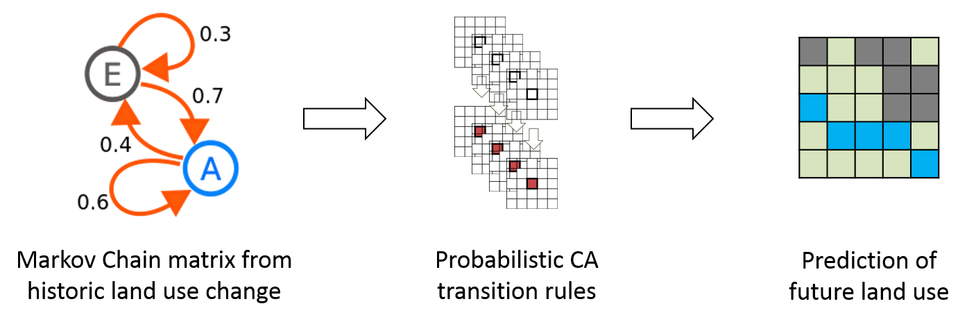
Figure 6.17: Probabilistic CA: the growth process is governed by statistical probabilities of land-use change.