Lesson 12 Parameterisation
Parameters are input variables. They adapt a generic model to a specific study area or use case. In the process of parameterisation a modeller thus needs to find the best fitting parameter values to represent a specific system.
Upon completion of this lesson, you should be able to
- calibrate a model,
- be aware of potential issues related to parameterisation, like overfitting, model sensitivity, uncertainty, or dependency between variables,
- quantify the robustness of a model against parameter uncertainty by means of a sensitivity analysis, and
- conduct Monte Carlo simulation to quantify the uncertainty in the model that is due to stochastic processes,
- avoid overfitting.
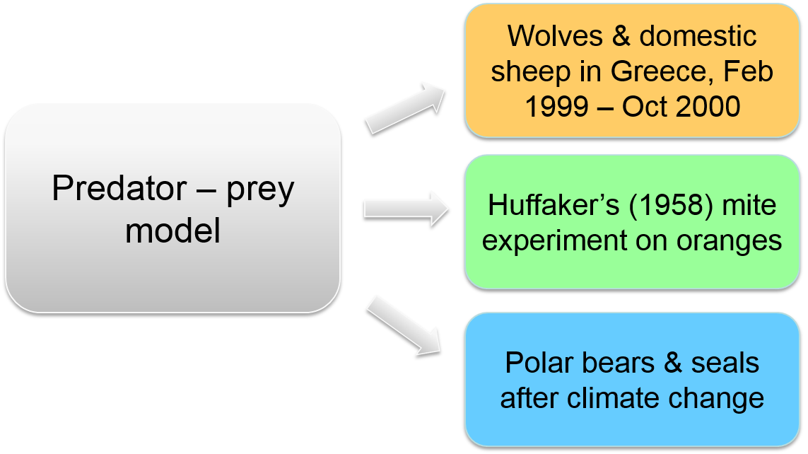
Figure 12.1: Parameters adapt a generic model to a specific question
To avoid confusion, here are some definitions on variables that we use in simulation modelling:
- Parameters are input variables. They describe the relevant properties of the system of interest and thus adapt a generic model to a specific modelling purpose and / or study area. They are like ‘independent variables’ in regression models.
- State variables output variables that describe the state of the system or an entity in that system at any time during a simulation. They are like ‘dependent variables’ in regression models.
- Other variables in the model can be global, local, cell, agent, random, non-random. These variables are ‘hidden’ in the model code and are not visible to the user of a model.
12.1 Choice of parameters
The first and most important step of parameterisation is to choose which parameters to include in the model and which ones to leave out. The Occam’s razor principle ‘less is more’ is fully valid in this case: less parameters often pay off in the usefulness of the outcome. So, the amount of parameters should be as low as possible without loosing a parameter that is essentially relevant for the modelling purpose. This step has been an important part of the conceptualisation phase. In the now following parameterisation phase, we need to assign adequate values to the chosen parameters.
12.2 Assign values to parameters
In the best case, a modeller knows the exact values of all parameters in the model for the specific study area of interest. Either because it is known from theory, or from empirical data. In this case parameterisation is a straightforward process and no further steps need to be taken. We then could proceed to run, analyse and validate the model.
In most cases parameter values are not exactly known. Instead, we just have an idea of the possible range of values that a parameter can take. In the worst case, the value for a parameter is completely unknown. For all these cases there are strategies for parameterisation. No matter, how sophisticated such parameterisation strategy is, we need to acknowledge that vague parameters increase the uncertainty of a model. The ultimate aim of parameterisation usually is not to find correct parameter values, but to reduce the corresponding uncertainty of the model.
12.3 Sensitivity analysis
So, what we actually want to know is the sensitivity of a model to parameter change: how much does any single parameter contribute to the overall uncertainty of the model result? Often there is a linear relationship: small parameter variations produce small changes in the overall results and large parameter variations result in large changes of model results. In the best case, there is some balancing feedback mechanism, so that the result does not change very much upon variation of the parameter and we do not have to bother about the exact value too much. In the worst case, a small parameter change entails large differences in simulation outcomes. A systematic test of how a model reacts to parameter change involves repeated simulations, each time with a slightly changed parameter over the entire range of its possible values. This systematic testing procedure is called sensitivity analysis and it is an essential part of model uncertainty analysis.
In extreme cases, when very small parameter changes have dramatic impacts on the model result, we talk about chaotic systems. The classic example of chaotic systems is a butterfly that strokes its wings in Amazonia and thus causes a hurricane in the Caribbean.
12.4 Calibration
Let’s consider a very common case of parameterisation: we have a rough idea of typical values that a parameter takes, but do not exactly know the correct value for the study area. That is, we need to calibrate the model against real data in order to fit the model to the study area. To do so, the model is parameterised with a set of possible alternative values. The alternative simulation outcomes are then tested against empirical values that were measured in the real system. The best fitting value is then assumed to be the ‘correct’ parameter. Importantly, we need to set aside empirical validation data that we do not use for calibration. Otherwise, we could not appropriately validate the model anymore.
12.4.1 Overfitting
A problem that is closely related to calibration is overfitting. An overfitted model describes random variations instead of the underlying relationship. It closely reproduces the system to which it was calibrated, but it cannot predict beyond its temporal and spatial extent or explain general system behaviour.
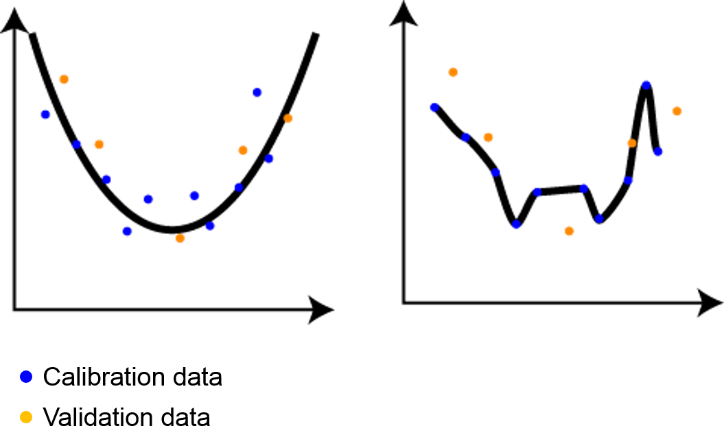
Figure 12.2: The aim of a model is to fit the underlying process (left), not to precisely ‘overfit’ the calibration data (right).
In Figure 12.2 we have calibration data (blue points) and validation data (orange points). On the left side, the underlying process is adequately captured and the model represents the validation data equally well as the calibration data: the model is well calibrated. The model on the right side is overfitted: if perfectly represents the calibration data, but fails to explain the validation data.
A strategy to overcome issues of overfitting is the approach of pattern oriented modelling that was introduced by Grimm et al. (2005). Pattern oriented modelling refers to a fitting to several aspects (‘patterns’) of a system at the same time. It assumes that this is only possible, if the underlying structure of the system is correctly represented in the model.
12.4.2 Dependent parameters
Another frequent issue of calibration is dependence between parameters. In this case it is not enough to test parameters one by one, but instead the combination of multiple parameters needs to be considered. For example, both parameters ‘water scarcity’ and ‘abundance of predators’ impact rates of successful reproduction. If one parameter is high, it slightly reduces reproduction. However, if both parameters are high, the effect on reproduction of prey animals may be catastrophic.

Figure 12.3: For a gazelle, the combined presence of a waterhole and a lion is fatal, whereas it could avoid lions reasonably well otherwise.
At this point, it is worth to consider that each single uncertain parameter added to a model heavily increases the model’s uncertainty. For example, let’s assume we have one vague parameter and test five alternative parameter values. The test results in five alternative model results. The same strategy with two vague parameters results in 5^2=25 alternative model results. For a model with 10 dependent and vague parameters, the calibration procedure would result in 5^10=9,765,625, almost 10 million of alternative results. The number of possible model results thus increases by one order of magnitude with each new uncertain parameter. In such cases, we might come to the conclusion that the conceptual model needs to be reformulated and some parameters need to be removed or changed.
12.4.3 Stochastic parameters
So far, we have discussed parameters that are not exactly known, but they nevertheless were assigned with fixed values. However, often parameters are modelled probabilistically, for example a specific animal in a population has a 50% chance to be either male or female. Especially, bottom-up models with hundreds or even thousands of distinct entities with individual attributes and adaptive behaviour need to be parameterised by using random distributions. In spatial models this includes randomness of location. Even if all other parameters were kept constant, spatial randomness would create stochastic model results with an endless number of possible outcomes. In contrast to deterministic models, we here refer to probabilistic modelling. Whereas mathematical models usually are deterministic, most simulation models are probabilistic.
12.4.4 Monte Carlo analysis
If we run a probabilistic model multiple times we get a range of different results: this range is the uncertainty range of a model that is due to its random parameters. To make sound conclusions about the nature of results we need to treat the model outcomes statistically. For example, in a population dynamics model that we simulate five times, the resulting numbers of animals in the population after a certain number of time steps may be 492, 473, 501, 489, and 477. What do these outcomes tell us? Statistically, it is not sound to work with these data. To report a reliable mean value, the model needs to be run 100 times and more with the same parameter settings.
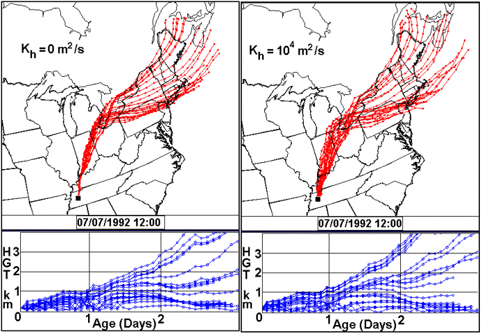
Figure 12.4: Monte Carlo simulation of a pollution plume (www.clear.rice.edu)
The implication of probabilistic models for parameterisation analyses is important: for probabilistic models it is not possible to directly compare two alternative sets of parameters. This comparison needs to be based on a statistical analysis of multiple simulation runs for each set of parameters. This systematic, statistical analysis to compare alternative sets of parameters is called Monte Carlo analysis. The result of a Monte Carlo simulation thus is a probability distribution of the outcomes of a multitude of simulation runs with the same settings. Consequently, the comparison of alternative parameterisations uses statistical tests to analyse differences in the probability distributions.
This sounds like a tedious way of modelling that entails a complicated model analysis. However, exactly in its stochastic nature lies the strength of agent-based models, which can directly represent random variation of individuals in a population, e.g. where each individual has a slightly different body size, age or sex. From this heterogeneity of individuals emerge new patterns that cannot be unveiled with deterministic models.
12.4.5 Reverse engineering
Finally, we face the most challenging case: we have no idea about the value a parameter might have. Still, it is possible to build a useful model, if we use the model to systematically calibrate the parameter against empirical data to find the best-fitting value. A problem that we might face in reverse engineering is called ‘equifinality’. Equifinality means that the multiple parameterisations can produce the same outcome. A strategy to best-as-possible avoid picking incorrect parameters in equifinal models is to test the results not only for one system state variable, but for a set of multiple state variables (see also ‘pattern oriented modelling’ approach that we have discussed before).

Figure 12.5: Reverse engineering is to ‘guess’ and systematically test, which parameter values could lead to the observed pattern
Reverse engineering has analogies to putting together a jigsaw puzzle. It comes at the cost of large model uncertainty. However, as long as we acknowledge the uncertainty, the model may still be useful to gain insights into a system. It lies in the hands of the modeller to argue on the validity of a model and consequently to defend its usefulness.
12.5 Exercise - batch experiments
Agent-based models and cellular automata are stochastic. Thus, the outcome of a simulation will vary each time that you run the model. In order to understand the nature and the magnitude of this variation, a modeller has to execute a model many times. It would be tedious to do this manually and note down the results after each simulation run. Batch experiments help to automate this process. In addition to recording results and restarting the model automatically, batch experiments can run in parallel on several kernels of your computer. Thus batch experiments are much faster than the manual (sequential) repetitions.
In this exercise you will work with an existing model and create your own ‘in-silico’ experiments to produce simulation results in a systematic and automated manner. This exercise is particularly useful for designing and conducting Monte Carlo simulations (many repetitions of the same experiment to see the effect of stochasticity in the model) and sensitivity analyses (systematic modification of a parameter to see, how sensitive a model reacts to small parameter changes).
12.5.1 Batch experiments
Consider a very simple model with only one variable my_var with a starting value of 0. Each time step the model adds 1 to my_var with a 50% chance.
model batchexperiment
global {
  int my_var <- 0;
  reflex add_1 {
    if flip (0.5) {
      my_var <- my_var + 1;
    }
  }
}
The simulation should run for 50 time steps and we repeat it 100 times. Which outcome would you expect?
To declare an experiment as a batch experiment you can make use of the facet type: batch. To automate this process you need to define the number of repetitions and the stop condition. For example:
experiment Monte-Carlo type: batch repeat: 100 until: cycle = 50 {
}
Now, there are two approaches to record the outcome of each simulation. Either you write the results to a file, or you collect the results and display them in GAMA.
1) Saving results to a file
First let’s consider we want to save the value of my_var for each of the 100 simulations to a .csv file. GAMA handles this as 1 model run with 100 simulations. However, we want to save the result not only once for a model run, but for each of the 100 repeated simulations. So we have to use a little trick. In a batch experiment GAMA offers a default species that is called simulations. We thus can ask simulations to do something, e.g. save the results to a file:
experiment Monte-Carlo type: batch repeat: 100 until: cycle = 50 {
  reflex save_results {
    ask simulations {
      save [self.name, self.my_var] to: "../result/be.csv" type: "csv" rewrite:false;
    }
  }
}
Note that you need to set the rewrite facet to false in order to keep all data entries. The pseudovariable self before the variables (self.name and self.my_var) ensures that each simulation saves its own variables.
Once you have saved your data to a .csv file, you can further process and analyse it e.g. with R or Excel.
Now it’s your turn: how would you go about to create a file with a nice header for the columns? You won’t need any additional command to do it. Actually it’s quite similar to how we saved the attributes. You just do it once, if the name of the simulation… Implement the model and see whether it works! If you want you can also post your solution to the forum.
2) Chart displays
In the second, alternative approach you can summarise the outcomes of your batch experiment directly in GAMA. To do so, GAMA offers the permanent statement. The permanent section allows to define an output block that will not be re-initialised at the beginning of each simulation but will be filled at the end of each simulation. To make full use of the permanent statement, we need a possibility to collect all the values that are produced in the repeated simulation for my_var. This is done by the collect statement. The syntax of the collect statement is as follows:
container collect each.my_varSo we collect each value of my_var from the a container of elements (e.g. a list, or a collection of agents, or simulation). As return value, we get a list with all the my_var values in that container. If we wanted to have the min value of a variable out of a set of repeated simulations, we can just write:
min (simulations collect each.my_var)So let’s say, we wanted to know the mean value of all my_var values after 100 simulations. If the number of repetitions is large enough, we would expect this value to be close to 25, correct? To test our assumption, we can produce a xy chart, where x is 0.5 (the 50% chance to add 1 to my_var) and y is the mean of the my_var values collected over all simulation runs:
experiment MonteCarlo type: batch repeat:100 until:cycle = 50{
  permanent {
    display mean_value background: #white {
      chart "Mean value" type: xy {
        data "my var" value: [0.5 , mean(simulations collect each.my_var)];
      }
    }
  }
}
Besides the xy plot, you can display also other chart types. Here is an example of several charts displayed on one tab.
permanent{
  display Stochasticity background: #white {
    // histogram
    chart "histogram" type: histogram size: {0.5,0.5} position: {0, 0} {
      data "<21" value: simulations count (each.my_var < 21) color: #green ;
      data "21-23" value: simulations count (each.my_var <= 23 and each.my_var >= 21) color: #green ;
      data "24-26" value: simulations count (each.my_var <= 26 and each.my_var >= 24) color: #green ;
      data "27-29" value: simulations count (each.my_var <= 29 and each.my_var >= 27) color: #green ;
      data ">29" value: simulations count (each.my_var > 29) color: #green ;
    }

    // data series
    chart "series" type: series size: {0.5,0.5} position: {0.5, 0} {
      data "my Var" value: simulations collect each.my_var color: #red ;
    }

    // xy plot
    chart "xy mean" type: xy size: {0.5,0.5} position: {0, 0.5} {
      data "my var" value: [0.5 , mean(simulations collect each.my_var)] ;
    }
  }
}
12.5.2 Sensitivity analysis
So far, we have played around with multiple repetitions of exactly the same model. However, to assess the sensitivity of a model to changes in its parameters, we need to compare repeated model simulations for different parameter settings. You can test this with our simple model above by introducing another parameter that governs the probability of which “1” is added to my_var at each time step. Let’s call this parameter chance and allow values between 0.0 and 1.0.
We can make use of a batch experiment to conduct an automated sensitivity analysis. To do so, we just have to define the variation of our parameter in the batch experiment:
parameter 'chance' var: chance min: 0.1 max: 0.9 step: 0.2;Now it’s your turn:
How many simulation runs will be computed, in the above case? Add the parameter to the model and run the batch experiment again.
Did you realise that the plots are re-initialised each time, when a new model run with a new parameter value is loaded? Only the xy chart summarises all the simulations for each of the five model runs (i.e. for each of the five parameter settings). Thus, we can make use of the xy chart to plot the parameter values (here: chance) against the respective summarised model outcomes (here: mean of my_var over 100 repeated simulations).
Congratulations! You have just succeeded in computing your first sensitivity analysis. Before you now go on to solve the assignment of this lesson, take a minute to think about the results: is the model sensitive against parameter change?