Lesson 13 Validation
It is an (unfortunately wide-spread) misconception that validation is something that happens in the end, after the model has been finished. However, validation is a process that needs to parallel model development. In fact, validation is the umbrella term for a set of procedures during model development that make sure that a simulation model fulfils its intended purpose: validation sensu stricto, verification, calibration, and credibility building (Rykiel Jr 1996). Each procedure can be mapped to a specific step in the modelling cycle:
- Verification is a demonstration that the modelling formalism is correct. Hence, verification is part of the formalisation step. Related testing strategies ensure that the code in agent-based models or the equations in system dynamics models are implemented correctly.
- Calibration is the estimation and adjustment of model parameters and constants to improve the agreement between model output and a data set. Calibration thus is a procedure in the parameterisation phase.
- Validation sensu stricto is a demonstration that a model within its domain of applicability possesses a satisfactory range of accuracy consistent with the intended application of the model. Validation is defined as the last step of a modelling cycle.
- Credibility is a sufficient degree of belief in the validity of a model to justify its use for research and decision making. Credibility is not part of the modelling cycle. The confidence of the modelling community into the validity of a model is built successively by a transparent and comprehensive description of a model, its uncertainties and the applied validation procedures. The credibility further increases over time, if the model is frequently used by different research groups and for multiple study areas.
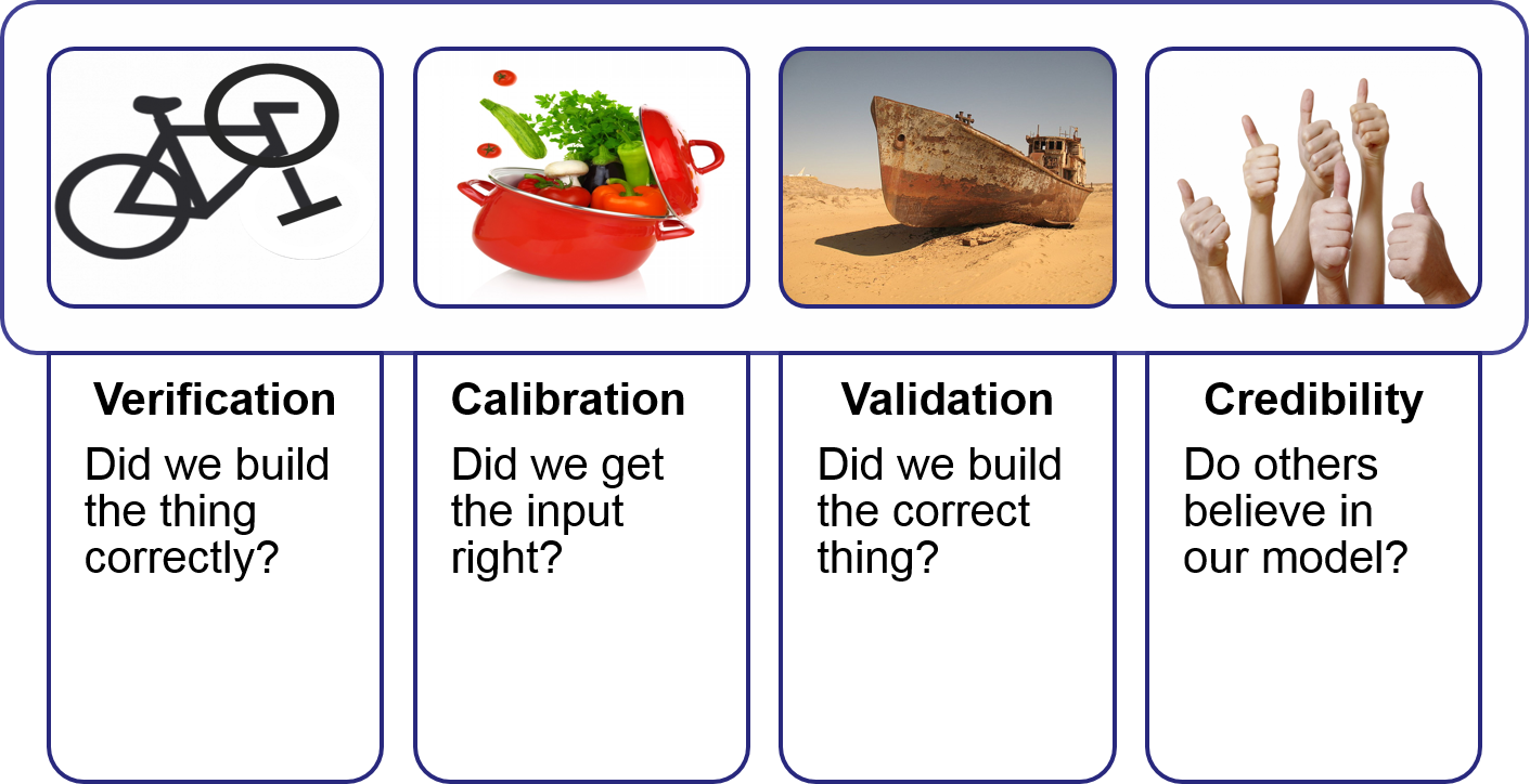
Figure 13.1: Validation has several aspects that all contribute to the overall model validity.
There is much debate in the literature about validation. Most authors agree that validation is an integrative part of modelling. Having said that, not all models need to be validated to be useful. Highly abstract models cannot be validated with empirical data, but still these models can be important tools in theory development [e.g. caswell1988]. On the other side, even very realistic models never can be ‘true’ in the sense that they perfectly represent reality. This would neither be possible, nor would it be useful. So the question is, how much abstraction do we want and how much ‘imperfection’ can we accept? Hence, validity depends on two things: the purpose of the model and its uncertainty. The third aspect of validation is the context, e.g. the geographical and temporal extent for which a model is designed.
In this lesson, we first have a look into these three aspects of validation: purpose (yes, again!), uncertainty and context. Then we will discuss some strategies and methods to test models and finally we will illustrate a validation workflow with an example.
13.1 Purpose
We start with an example from our everyday lives – the weather forecast. Let’s assume that the weatherman in TV predicts that the temperature will decrease by 5°C from 25°C at the present day to 20°C at the next day. He further explains that for some meteorological reasons this prediction is highly uncertain with an uncertainty range of +/-10 °C, so that the predicted temperature ranges between 10° and 30°C. Pretty bad model, isn’t it? So, is this forecast model still valid?
You will have guessed the answer: whether this forecast is valid or not, depends on the purpose that you have defined.
- Did you watch the weather forecast in order to decide, whether you want to go to the beach? Probably, the weather forecast model was not a great help with this decision. Or with other words: it was not valid for your purpose.
- Or does it suffice to know that tomorrow it won’t freeze, so that you do not have to bring the plants indoor? In the latter case, the model is highly uncertain, but it is still valid for your purpose.
Weather forecasts are an example of predictive models. The purpose is to predict the future state of a system as closely as possible, but it is not important to understand the underlying structure and processes. Often, these models depend on a vast amount of data and observed probabilities of change. The relevance of such models has increased dramatically with the high abundance of (real-time) data from many sources: satellite data, social media data, sensor webs, monitoring facilities, etc. Especially in urban areas, the pulse of human life can be accurately measured and predicted based on sources such as mobile phone data, twitter data, floating car data, air quality control sensors, or webcams. Smart city initiatives use these data together with big data analysis for predictions to ‘smartly’ manage a city: where to position policeman during an event? How to redirect commuters traffic to avoid congestions? Which places are tourist hotspots to efficiently advertise a touristic event? For all these questions, we do not care why people behave as they do. It is sufficient to know that they will behave this way in order to take adequate management measures. Validation methods therefore concentrate on prediction uncertainties.
In scientific models, a scientist conceptualises new ideas about the structure and processes that define how a system ‘works’ in a model. In this context, a model is nothing else than the formalisation of a narrative, e.g. how animals establish their territories, or how fish interact when swimming in schools. Hence, scientific modelling is a way of abductive reasoning: it starts from an idea of how a system might work, which is then formalised into a model to be tested. The model itself equates to the formalised hypothesis. Validation strategies concentrate on the validity of the internal structure of a model. Two broad categories of scientific models can be distinguished:
Empirical models If the model is specific enough to be parameterised with real-world data, it can also be validated with empirical data. If the model then fails to reproduce real-world patterns, the hypothesis is incorrect or an important aspect of the system is missing. However, the inversion of argument would be erroneous: a hypothesis is not necessarily ‘true’ upon successful validation. This is due to the problem of equifinality, which states that the same pattern can result from multiple alternative processes. Global climate change models belong to this category.
Theoretical models If a model is too abstract to be used in a real-world context, other (weaker) validation methods can be applied. This is often the case in theory development, where the modeller aims to compare patterns that result from several alternative structures and processes. Such theoretic models usually have a simpler structure in order to have a generic and crisp relationship between processes and patterns. The Game of Life models are a prominent example in this category.
13.2 Uncertainty
Many definitions for uncertainty exist, here are some of them:
Uncertainty is not just a flaw that needs to be excised (Couclelis 2003)
Uncertainty is an intrinsic property of geographic information (Duckham and Sharp 2005)
Uncertainty is the umbrella term of these imperfections (Longley et al. 2005)
The common denominator of these definitions is the view that there is nothing wrong with uncertainty. It is a natural part of any (geographic) information. However, it is important to know how uncertain our data is in order to adequately use it. In simulation models the assessment of uncertainty is not a trivial task, especially when it comes to uncertainties in the structure of a model. A good starting point to think about uncertainty analysis is the ISO standard 19157 “Geographic Information – data quality”. According to this standard, there are five components of spatial data quality:
- Attribute accuracy
- Positional accuracy
- Logical consistency
- Completeness
- Lineage
In another, a more epistemological view on uncertainty, we can think of three domains:
| known knowns | describe what we know about a system |
| known unknowns | are all aspects that we are uncertain about: we know that they are there, but we do not know, why and how they operate. These known unknowns are subject to potential hypotheses. |
| unknown unknowns | These are the most unpleasant companions. We call it ‘noise’ or ‘random variation’ and have no explanation, where it comes from. |
Scientific models aim to add to the known knowns by finding explanations for known unknowns. For example, we know that there are still unexplained carbon sinks in the global carbon cycle and there are a couple of alternative hypotheses where to find these. Carbon cycle models have not yet fully unveiled these mysterious sinks. Eventually scientific models even discover an unkown unknown, if unexpected patterns are detected. However, they are most probably often overlooked, because we do not even have a clue that we could look for them.
13.3 Methods for validation
When we want to assess the quality of a model, we can reflect on its structure (e.g. the entities, their attributes and behaviour or how processes are scheduled and updated), its input data (e.g. the initialisation data or the parameters) or its output (state variables and patterns). Whereas structure and data are tested in the beginning of the iterative modelling cycle, the test of a model’s match with the observed reality relates to an analysis of the output.
As a simulation model is a complex representation of a system, there are uncountable number of potential outputs, i.e. views that can be taken on the system. Instead, we need to explicitly choose in which aspects we are interested and which indicators can best describe the aspects of interest. A possible (quantifiable) indicator can be a system-level state variable that describes the current state of a system. We can choose the value of the state variable at the end of the simulation or the time series of values to describe its temporal dynamics over the entire simulation. Further, we can aggregate state variables of individual agents, e.g. over time, over space or over different agent types. Finally, we can choose a set of indicators that together describe a particular (spatial) pattern. For example, in a flocking model the birds in a flock could be aggregated to characterise a flock by its number of birds, the mean nearest neighbour distance between birds in the flock, and the standard deviation of flight directions.
Now, that we know about a model’s potential purposes and aspects of its uncertainty, we can start having a look into methods for testing procedures. According to Rykiel (1996), there are three levels of validity.
- Conceptual validity states, whether the underlying theories & assumptions are correct
- Data validity states, whether the model simulates realistic outcomes. However, data validity does not imply that the underlying conceptual model is correct (issue of overfitting).
- Operational validity states, how well the model outcome represents the observed real system.
![An overview of available testing methods in the validation process after Rykiel [-@rykiel1996].](images/testing-methods.png)
Figure 13.2: An overview of available testing methods in the validation process after Rykiel (1996).
In the diagram above (see Figure 13.2), levels of validity are categorised according to the theoretical understanding of how the system functions (x-axis) and the availability of validation data (y-axis). For each validity level a set of adequate testing methods are available (see Rykiel Jr 1996). In the remainder of this lesson, we will have a closer look at these tests. Many of them are common sense. However, only an overall testing strategy that orchestrates single tests to a rigid workflow makes sure that a model can live up to its expectations.
13.3.1 Face validity
As modellers we often work together with domain experts, e.g. biologists, geologists, or geomorphologists. These experts are probably as eager as we are to see first results. Experts can give valuable input, especially at the early stages of model development, where more rigorous and data-based testing methods cannot be applied. Therefore testing starts right away, with the validation of the first conceptual model. At this stage the face validity method tests, whether an expert thinks that the model ‘looks like’ it does what it should. That is, whether the structure appears reasonable ‘on the face of it’ and whether the model is likely to simulate the expected outcome given the model’s purpose. Although, face validity tests often trigger valuable inputs, we need to be aware of the high subjectivity of this test.
13.3.2 Event validity
After the first round of a modelling cycle, when we have simulated the first results, we probably have a wealth of good ideas how to improve the model. However, it is a good idea to withstand the temptation to fix this and that and instead take again time for validation. In a qualitative comparison between the simulated outcome and the real system, we can establish event validity: how well does the model simulate the occurrence, timing and magnitude of events? At this early stage, we cannot expect that the model reproduces system behaviour quantitatively correct. Instead we focus on relationships among model variables and their dynamic behaviour.
13.3.3 Turing test
As the understanding of the behaviour of our model increases, we can still apply tests for face validity and event validity, but also include more rigorous tests of the conceptual validity. A famous qualitative test is the Turing test. It is named after computer scientist Alan Turing, the father of artificial intelligence. In a Turing test, two visualisations are presented to an expert: the outcome of a simulation and the representation of the real system. If the expert cannot spot the simulation, the model has passed the Turing test.
13.3.4 Model comparison
A popular test, for frequently studied systems is a comparison between models. In some cases, as for example for global climate models, this may be the principle means of validation. The idea behind this approach is simple: models that build upon the same conceptual understanding, and only differ in the way of implementation are expected to produce similar results. If model results are similar compared to each other, but differ from the real system, the conceptual model needs revision. Later in this lesson, we will discuss benchmarking, a validation strategy that has evolved from this approach.
13.3.5 Traces
Finally, traces can be analysed through simulation runs. Traces are specific state variables that describe a relevant process. To plot a graph of state variables over time is a standard procedure, which is facilitated by all common modelling frameworks. The critical point here, is the selection of the essential processes and related state variables.
13.3.6 Statistical validation
A critical factor in model calibration and validation is the abundance of adequate data that is available for validation. Statistical analysis is essential for any quantitative validation of a model and without rigorous statistical testing, a model cannot be claimed to be ‘realistic’. For model calibration, multiple simulation runs with alternative parameterisations may be tested against empirical data to determine which parameters fit best. Of course, the data that is used for model calibration cannot be used for validation. Statistical validation usually tests whether the simulated data are significantly different from the real data. Adequate statistical testing procedures to compare two sets of data belong to the family of ‘t-tests’. Potential significant differences can be further described by comparing statistical properties such as mean, median, range, distribution or bias. Even in case there are significant differences, there might be acceptable limits for this error. Finally, as we are focussing on spatial models, it is recommended to use methods from spatial statistics to specifically test for spatial properties of interest. In the upcoming lesson on scenario-based research, we will have a more detailed discussion of adequate methods of (spatial) statistical methods for quantitative model analysis.
13.3.7 Operational validity
The most rigorous level of validation is the ‘operational validity’. Operationally valid models are based on both, a sound theoretical understanding of system structure and processes and rigorous statistical testing with empirical data. All validation techniques discussed so far are the basis to conclude operational validity for a model. A comprehensive framework to achieve operational validity is ‘pattern oriented modelling’ (POM) (Grimm et al. 2005). POM suggests to use a meaningful set of state-variables (=patterns) for the comparison between model results and real-world data. The idea behind this approach is that a model can easily be tuned in a way to reproduce one state-variable. However, it is hardly possible to reproduce a set of independent state-variables at the same time just by tuning parameters. If all aspects of a pattern are well reproduced by the model, this means that the model’s structure correctly resembles the real-world. Although operational validity is the ultimate goal for any model, the focus differs with the purpose. Whereas predictive models strive for strong data validity, scientific models focus on conceptual validity.
13.4 Summary
Validation is not something that is to be kept until the end, but it is a core part of the iterative modelling cycle. A multitude of testing strategies exist for various stages of modelling as well as for addressing different modelling purposes (e.g. for prediction or for understanding). However, the final validation of models that work with real-world data is to check operational validity by the means of pattern-oriented modelling.
Two things to remember:
- the definition of the kind of patterns that you are going to test at the end are part of the very first conceptual model
- The model cannot be more accurate than your validation data are (shitty data -> shitty model!)