Lesson 9 Agent-based models
In order to understand the nature of agent-based models and to be able to design such models, in this lesson we decompose an ABM into the three core components of a system: purpose, elements and interrelations. Especially, the adaptive behaviour between smart living agents governs the emergence of complex, self-organised systems and swarm intelligence. Given that interaction only can happen within a local neighbourhood, spatial configurations are a key structural element of such living, complex systems.
Upon completion of this lesson, you will be able to
- identify, whether an Agent-based model is an adequate choice for a particular use case,
- design agent-based models in a structured way, according to decision-making theory,
- apply the four steps of a decision making workflow (perceive environment - sense inner state - decide - act) to represent behaviour, and
- understand, how the choice of spatial neighbourhood concepts to represent perception and action impacts model outcomes.
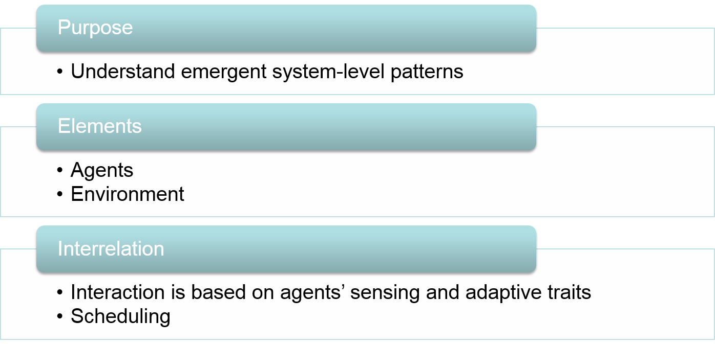
Figure 9.1: A conceptual overview of the agent-based modelling approach.
9.1 Purpose
The purpose of agent-based models is to explain large-scale patterns with the adaptive behaviour of interrelated individuals. System-level properties like population size, birth- and death rates are the result rather than the input.
Agent-based modelling is thus an adequate tool, if we know a lot about the behaviour of individuals and wonder about the collective behaviour.
In the Life Sciences, agent-based modelling has gained momentum for its close resemblance of living systems, where the core units of an ecosystem are individual animals and plants. An animal for instance is not aware of any birth-rates at population-level. Actually, it will successfully give birth to offspring, if it finds a mating partner at due time, and if there is enough food around the nest for feeding.
The notion of emergence is important for agent-based modelling: ‘not easily predictable’ does not mean ‘impossible to understand’. In contrary, it is the primary goal of an agent-based model to unveil the mechanism of how system-level properties emerge from individual behaviour. If individual behaviour directly determines system-level behaviour, this would be an imposed behaviour – and we would not be able to learn anything from such a model.
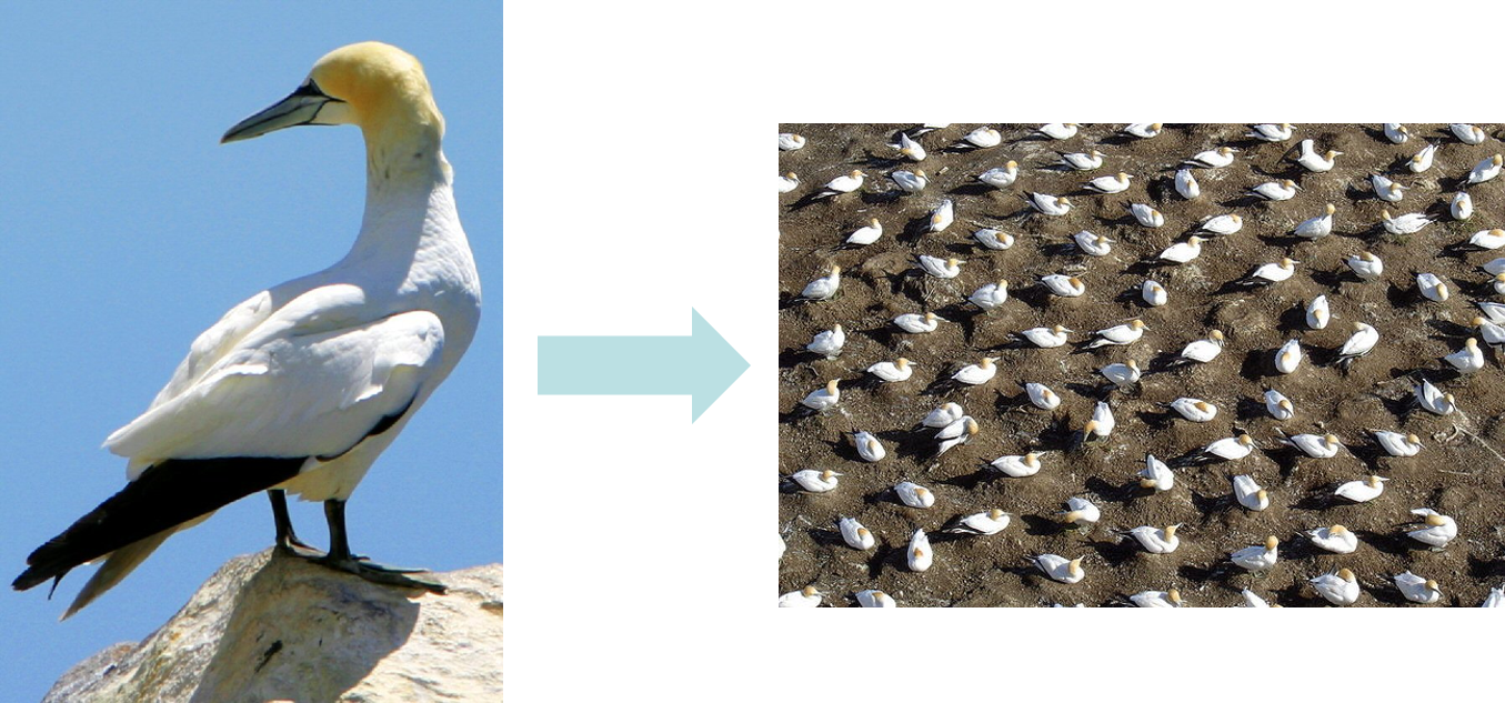
Figure 9.2: The uniform distribution of bird nesting sites can be understood by its generation: birds try to maximise the space around their nests.
9.2 Elements: agents
Just like in the movies, an agent in an agent-based simulation model is a discrete and autonomous entity that acts independently in reaction to its living and non-living environment. In the simplest case, agents are plants, but agents can also be animals or humans that actively pursue a goal, have a memory and are able to learn and to adapt.
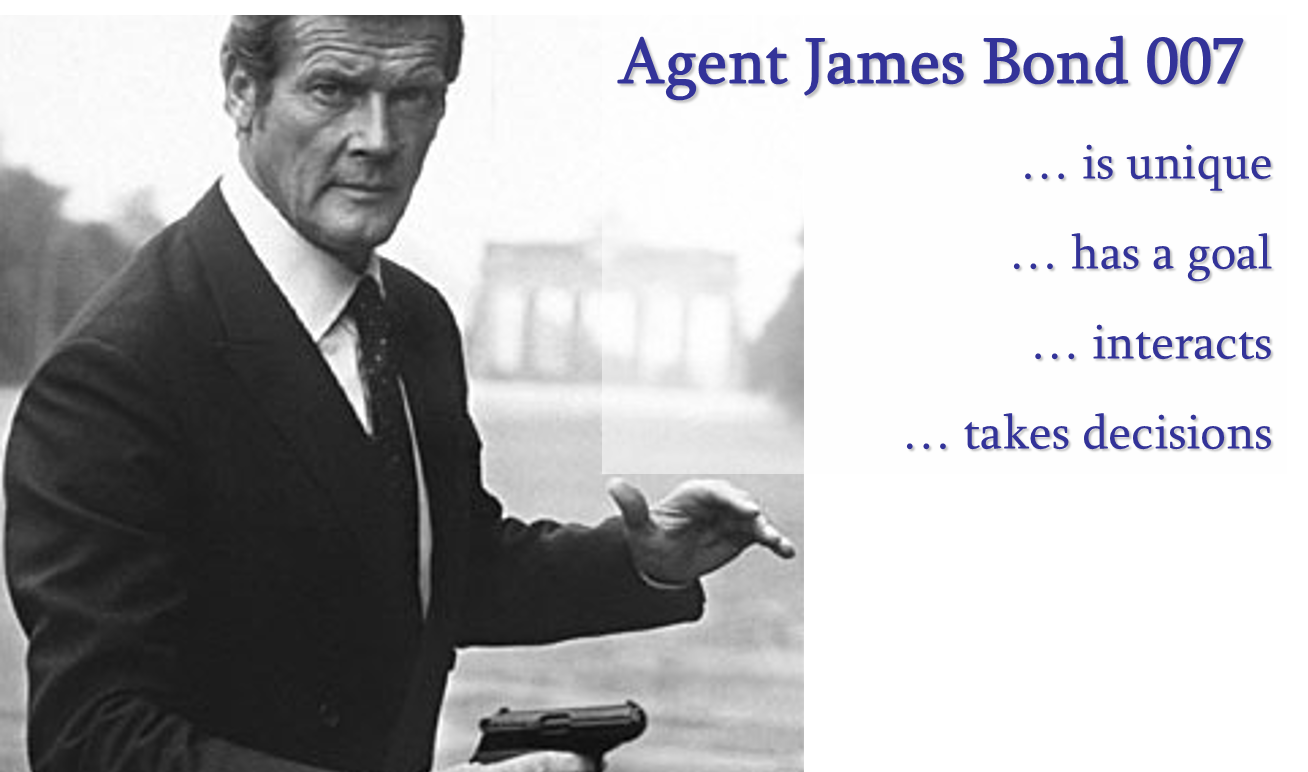
Figure 9.3: James Bond is an agent: he is a unique person that pursues the goal to save the world, he always takes the right decision in difficult situation and he shoots the bad guys and saves the women. Agents in an agent-based model have comparable properties.
From a computational perspective, agents are the basic building blocks of agent-based models. They are usually formalised as software agents in an object-oriented programming (OOP) language, in which discrete ‘agents’ (objects) are described with their potential behaviour (in OOP-terms referred to as methods or functions). The object-oriented programming paradigm is a natural fit for agent-based modelling, because we can describe individual agents as an instance of a particular agent type (in OOP referred to as a “class”), where each agent is created following the same class-blueprint. This means that each agent has the same attribute-types (e.g. age, gender, size) and the same behaviour-types (e.g. moving, eating, communicating), but the actual values can be specific to each individual. This concept of a class (an agent type) being the blueprint for individual objects (the individual agents) is a central paradigm of OOP called “inheritance”. Typical OOP languages are Java, C, but also python has object-oriented features. GAML, the “GAma Modelling Language” is an OOP language that was inspired by Java and has been optimised for implementing agent-based models especially by non-computer scientists.
9.3 Relations: behaviour
Cow agents feed on grass, lion agents eat zebra agents and pedestrian agents stop by to have a chat with another pedestrian agent. Such typical behaviour is implemented in an ABM as a set of if-then-else rules.
Behaviour is basically expressed by a set of “if-then” decisions rules that define the circumstances under which a specific agent decides to take specific actions to meet a specific purpose or goal. Behavioural rules can either be derived from theory (theory based models) or from empirical data (data driven models).
The set of predefined decision rules is the blueprint that describes the behaviour of a certain species or a certain type of a human population. Although, all agents of the same agent-type “own” the same potential behaviour, their individual actions differ with respect to their specific spatial and temporal context, because each individual has different inner states, different locations and thus different external cues in its local environment, and different scheduled agendas, e.g. depending on its age and sex. The spatial environment in which agents are located typically is a dynamic landscape that is modelled by means of a cellular automaton.
To a great extent, the individuality of agents is rooted in the explicit consideration of space: the specific spatial configuration of other agents and the heterogenous environment at an agent’s location. In addition, there is some stochasticity due to individual variations and preferences.
From a geographical point of view, agent-based models opened the possibility to study the evolution of systems from a spatial perspective. An influential model towards this end was the implementation of the traditional system-dynamics model on predator-prey systems in the form of a spatially explicit agent-based model. The spatial predator-prey model has triggered an increasing interest in the spatial distribution of animals (e.g. Wilson et al. 1993). Heterogeneous spatial configuration of the environment was found to have a stabilising effect on population dynamics (e.g. Crowley 1981). Spatial territories emerge through species interactions (Potts and Lewis 2014) and habitats emerge from species competition for resources (Grimm and Railsback 2013).
Expanding on the description of individual behaviour, we can define social behaviour as a set of rules that describes whether and which actions an agent of a specific population takes, if it perceives the presence of another agent. This can be interactions between individuals of the same agent type (e.g. flocking birds), or interactions between different agent types (e.g. predator-prey).
9.4 Decision making
Smart, living agents permanently take decision what to do next given the current situation. These decisions are taken fast and mainly subconsciously. However, in agent-based models, this iterated decision making process needs to be made explicit. To model this process in a systematic, task-oriented and comprehensive manner, it is helpful to relate to some decision-making theories for the design of models, even if we were to parameterise the model in a data-driven approach.
we visit the idea of bounded rationality (Simon 1990): in contrast to the perfect decision that is based on full analysis of data from the entire system, an agent always only can decide based on the fraction of the system it perceives. This bounded rationality may lead to sub-optimal decisions of individuals. In contrast to aggregated models, agent-based models are particularly well suited to represent this omnipresent phenomenon.
there is the Observe-Orient-Decide-Act (OODA) loop that was suggested by the United States Air Force Colonel Boyd (1976). The OODA loop is a military decision strategy that was developed for combat situations, which ask for rapid decision making. The OODA loop has become popular also in fields beyond military applications. Due to its fast and efficient approach to decision making and its incorporation of bounded rationality the OODA loop lends itself especially well for implementation in agent-based models.
the Belief-Desire-Intention (BDI) framework is based on the theory of human reasoning (Bratman 1987). This theory served as the foundation of the belief-desire-intention architecture to programme intelligent agents: an agent has a certain belief of its environment that is framed by its only restricted ability to observe the environment and it has a desire of what to achieve on the long run. The intention of what to do next is based on its belief and its desire.
the ecological concept of adaptive traits considers all the attributes and decision rules that define an agent’s potential behaviour together as a trait. This is the “biological rule set”, which the agent has at hand for decision making and acting. Adaptive traits are traits that have evolutionary adapted the species to perform well in its specific environment and to take full advantage of its ecological niche. All animals in a population share the same (adaptive) trait, e.g. their behaviour in danger: mice flee, toads bump air into their body to appear bigger, bees sting, beetles act as if they were dead and chameleons camouflage themselves. However, whether or not an individual bee stings, depends on its age, the weather, the time of the day and its current mood.
In summary, the common denominator of all these decision making theories for animals and humans alike, involve four activities through which an agent’s iterates each time step:
- The agent senses its environment,
- queries its inner state and memories,
- takes a decision on what to do next, guided by its general goal(s) and based on the gathered information, and
- (inter)acts.
9.4.1 Sense the environment
This first step of the decision making workflow, through which an agent iterates each time step, is the perception of the environment. To understand the state of the surrounding environment, an agent uses all its senses, including seeing, hearing, feeling, and smelling.
A model in the simplest case aggregates all senses into one (often) circular buffer that ignores spatial heterogeneity. This can be a good, first approximation that consumes a minimum of computational power. It is a valid approach in abstract models or in cases, in which there is not much known about the perception capacities of a species.
Why should we bother about more realistic representations of the perception process? Or in other words: how much can we expect a model outcome to change, in response to different ways to model perception neighbourhoods? Check it out in the following exercise on perception neighbourhoods!
Exercise: perception neighbourhood
In the NetLogo model of this exercise (Figure 9.4), an ant moves in a landscape. The environment consists of a toroidal space that wraps around itself endlessly in all directions. In the centre, there is a hill and on the eastern hillside, there is a wall. The ant senses its environment (area covered in blue) and then randomly selects a location within the perceived area.
There are 3 implementations of perception neighbourhood that you can choose from:
- circular buffer, ignoring the heterogeneity of space
- angular buffer (a forward-looking cone), also ignoring the terrain
- angular viewshed, considering the terrain
Instructions
Explore how the virtual ant in the perception-neighbourhood model (Figure 9.4) moves around with respect to the different neighbourhood concepts: setup and run the model for 1000 time steps (go 1000) and note down the resulting travelled distance. You may want to move the speed slider to have the simulation run quicker.
Question
Do the trajectory patterns and the travelled lengths differ between neighbourhood concepts, and if so, can you explain why?
Figure 9.4: Explore, how different local process neighbourhoods impact the system-level outcome, NetLogo Web
Solution of the exercise.
Cirular neighbourhood
The circular neighbourhood results in random movement. The hilly environment and the wall do not influence the movement, because the circular buffer that approximates the ant’s perception simply ignores the environment. The result is a random walk pattern.
Angular neighbourhood
In this case, the perception is restricted to a forward directed cone. It results in a trajectory with a more consistent direction, which appears to be more realistic. However, if you would zoom out by one level of scale, the movement would still be random, thus this pattern is called “correlated random walk”. The travel distance is the same as for a circular perception neighbourhood.
Viewshed
In this third case, the geographic environment is considered. The ant only can move to a location that it can see. The total travel distance is less than for the (correlated) random walk, because the animal can only go as far as it can see.
You may have realised that the ant quite frequently goes along the top of the wall, and sometimes even crosses it. This is because, we have restricted the perception, but not yet restricted the action neighbourhood: the ant can go to any place it can see from its current location.
Unfortunately, Agent-based models that are reported in the literature almost never make use of viewsheds, or other more sophisticated geographic representations. The reason simply is that these features are not implemented in ABM software (yet). Netlogo has no off-the-shelf possibility to represent viewsheds. Thus, I had to implement an algorithm from scratch for the NetLogo perception neighbourhood model. This asks for complicated code that most likely is computationally not very effective.
GAMA supports the computation of a vision blocked by 3d vector objects with the masked_by operator. Further, GAMA supports - unlike NetLogo - vector operations. With GAMA it is thus possible to represent perception neighbourhoods with circles, cones or other polygons.
Exercise: perception neighbourhood in GAMA
In this exercise we implement the perception neighbourhood concept into GAMA. Due to the lacking support for modelling viewsheds, we restrict ourselves to circular and angular buffers. As these two perception concepts ignore geographic space, we don’t need to model the hill and the wall, either.
Instructions for the circular buffer
With the following instructions, you should be in the position to code the GAMA model.
- Setup a new model.
- Create an agent of a species with the skill “moving” that walks around randomly.
- Declare a global variable for the perception distance.
- Create two visualisation aspects for that species: one for the species location with size 1, and one for the perception neighbourhood with the size of the perception distance.
- Draw the trajectory by
- declaring an empty list of point-locations as agent variable
list<point> trajectory <- [];to which the current location is added at each time stepadd location to: trajectory;, and - drawing the trajectory as line feature in the agent’s aspect
draw line(trajectory) color: #black;.
- declaring an empty list of point-locations as agent variable
- In the experiment section add a map display in which you visualise the species twice, once for each aspect. Add a transparency to the perception neighbourhood with the transparency facet:
species ants aspect: perception transparency:0.1;. - Add a second species that walks in correlated random walk, and visualise the arc of the perception neighbourhood:
draw arc(2*vision, heading, vision_angle) color: #limegreen;
As always, the solution is provided below, but try yourself first!
View the model code.
model Ex_L7a_perception_neighbourhood

global {
    // the radius of the perception neighbourhood
    float vision <- 7.0;
    float vision_angle <- 120.0;
    init {
        create ants_circle number: 1;
        create ants_arc number: 1;
    }
}

species ants_circle skills: [moving] {
    list<point> trajectory <- [];

    reflex ant_move {
        // random walk
        do wander;
        add location to: trajectory;
    }

    aspect ant {
        draw circle(1) color: #black;
        draw line(trajectory) color: #black;
    }
    aspect perception {
        draw circle(vision) color: #grey;
    }
}

species ants_arc skills: [moving] {
    list<point> trajectory <- [];

    reflex ant_move {
        // correlated random walk
        do wander amplitude: vision_angle;
        add location to: trajectory;
    }

    aspect ant {
        draw circle(1) color: #green;
        draw line(trajectory) color: #green;
    }
    aspect perception {
        // draw an arc with the diameter (the GAMA documentation says "radius", but it needs to be the diameter), the heading and the width of the vision's angle.
        draw arc(2*vision, heading, vision_angle) color: #limegreen;
    }
}

experiment simulate type: gui {
    output {
        display map {
            species ants_circle aspect: perception transparency:0.1;
            species ants_arc aspect: perception transparency:0.1;
            species ants_circle aspect: ant;
            species ants_arc aspect: ant;
        }
    }
}
9.4.2 Query the inner state
Perception of inner state, e.g. hunger, pain, state of healthiness, curiosity, energy level, hormone levels, emotions, memories. Models of the inner state probably are richer for humans than for animals or plants, but the principle is the same. Whether all inner states need to be queried depends on the modelling task. Evacuation from emergency situations reduces the number of relevant inner states to a survival-oriented minimum, whereas the choice of leisure time activities needs to be based on a richer set of state attributes.
Part of an agent’s inner state is also its memory. Learning and reference to memories entails the possibility to query the history of states. More on that in the next lesson.
9.4.3 Decide
Decision making is governed by the overall goal(s) of an agent. In this step, the agent trades off which overall goal it pursues, based on the perceived state of the environment on its inner state (including memories). The decision to take a specific action may then be triggered a) by an agent’s inner state (if I am tired, I go home), b) by an external cue (if it rains, I go home), c) by a scheduled agenda (if it is 5pm, I go home), or d) a combination thereof (if it is 5pm, and the sun shines, and I am not tired, I go for a walk. Otherwise I go home).
Smart agents behave in a way to react and adapt to a situation. Thus, agents need to take situation-dependent decisions. Such adaptation involves a set of rules, and also rules to change rules. For example, a wolf-agent might follow a rule “if I am hungry and a sheep-agent is nearby, then I kill and eat the sheep”. Accordingly, a car-agent will follow a rule “if the traffic light turns green, then I continue driving towards destination”.
To be more realistic, behavioural rules can be more sophisticated. For example, a wolf-agent that is nearby a sheep might trade off its level of hunger against its fear of being spotted by the shepherd dog. So the presence of the shepherd dog can change the behaviour of the wolf.
Agents might also be able to learn from experience. A wolf that has been bitten by a shepherd dog once, tries to avoid dogs in the future. Agents’ learning abilities involve ‘memories’ of individuals.
Sometimes, interaction rules are not deterministic, but they mimic a stochastic process. For example, the wolf that wants to kill and eat the sheep might only succeed with a probability of 80%. The variability at system-level emerges from such stochastic behaviour as well as the spatial distribution of agents that interact locally, adapt to the local environment and have individual learning experiences.
Let’s develop a use case with the ant model of Figure 9.4.
Exercise: decisions of a hungry ant
In the NetLogo model of this exercise (Figure 9.5), we assume that the ant has two competing goals: One goal is to find food, if it is hungry, and the competing goal is to hide from predators. We further assume that the food most likely can be found in medium elevations, whereas shelters are more frequent at the bottom of the hill. The ant thus will prefer certain elevations depending on its inner state.
To operationalise the decision making of this model, we implement the following rules:
- Each time step the ant consumes 1 unit of energy for movement.
- Each time step that it spends in medium elevations between 70m and 95m, it will be able to find food and thus win 5 units of energy.
- The ant gets really hungry at energy levels below 15 units. It leaves the shelter and moves upwards (=one of the five highest patches within its perception neighbourhood) to the food grounds.
- At medium energy levels, it stays in the medium-elevation foraging grounds, but only if it is already there, otherwise it stays sheltered.
- It will stop feeding and return downwards to a more sheltered neighbourhood at energy-levels above 50 units.
- To visualise the inner state of the ant, it will turn red when it is hungry (below 15 energy units), then orange (between 15 and 50), and finally green (above 50).
Instructions
Setup and simulate 1000 time steps of the decision-making model (Figure 9.5) for the different neighbourhoods. Compare the emerging movement patterns.
Questions
- Why does the ant quite often get “trapped” in the case of a circular neighbourhood?
- Describe the emerging pattern for the angular neighbourhood model.
- How do the emerging patterns for the viewshed neighbourhood differ?
Figure 9.5: Decision making is a rule-based trade off of goals that is governed by the state of the perceived environment and the inner state of the agent, NetLogo Web
Solution of the exercise.
Trapped, when perceiving a circular neighbourhood
The ant perceives its local neighbourhood, selects the ideal location and moves there. As long as it pursues the same goal, chances are high that the location it comes from is also amongst the best locations. So it turns 180° and starts moving forth and back and it is trapped in its local optimum. This is called a “lock in” situation in system science.
Emerging patterns, when perceiving an angular neighbourhood
In this case, the perception is restricted to an arc (=a forward directed cone). Therefore, the ant cannot turn round, but it keeps going. Although the location may be suboptimal locally, the ant may find even better suited locations elsewhere.
In the nicely emerging pattern, you can see that the ant stays where it is as long as it is in its “orange” food-mood between 15 and 50 energy units: either traversing the hill in mid-elevations, or staying sheltered at the bottom. It transitions between these sites only if it is hungry (red) or not hungry (green).
Emerging patterns, when perceiving an angular viewshed
The restricted perception narrows down the possibilities for the ant, so that it has to make smaller steps into sometimes sub-optimal locations. This is a good example of bounded rationality: decision making that has to operate with the restricted information that is available.
9.4.4 Act
An action is what an agent actually does in the forthcoming time step to put its current decision into practice. In other words: the action is the operationalisation of an agent’s decision for the particular time step, based on its inner state and on what it has sensed in its neighbourhood. An action can be movement, but also feeding or changing an inner state.
Scheduling is the chronological order in which activities are executed. A particular challenge hereby is to find the best way of representing concurrent behaviour. Strictly speaking, concurrent behaviour cannot be modelled, as a computer is not able to perform ‘multi-tasking’, unless we split the model to run on multiple cores. Such parallelisation has the potential to speed up the execution of a simulation, but it also brings along new challenges of how to divide and orchestrate modelling tasks. This is a story on its own, outside the scope of this module.
Exercise: turn a plan into action
To implement the decision-making model of the last exercise, we actually had to already also implement action.
Instructions
Go back to the NetLogo decision-making model (Figure 9.5) and switch into its code tab, to see how individual actions are implemented:
- the
to goprocedure (lines 64 - 75) sets the order of procedures that are followed each time step: perceive - sense - decide - the
to decideprocedure (lines 147 onwards) encodes the decision rules that govern the behaviour of the ant
Question
- Check line 156 in the
to decideprocedure. Which actions are triggered here: “if I am hungry and I am below 70m”? - What is the order of actions. Does it matter?
- Look into the action that implements the decision to “go upwards” in lines 206 - 216. How is this action implemented?
- For this particular case, what is the goal, the decision and the action?
Check your answers!
What happens, “if I am hungry and I am below 70m”?
- Two actions are triggered: first, the ant turns red (
update-colour (red)) and then the procedurego-upwardsis called.
The order of actions
- First, the colour changes to red (indicating the state of hunger), then the go-upwards action is called. This sequence makes sense, because hunger is the trigger for the upwards move. It would not make sense to first let the agent move and then visualise the state change. However, in this particular case, the go-upwards action only prepares movement, the move itself is executed after the decision-making process (see next question for details). The user would thus not notice the difference.
How is to go-upwards implemented?
- The ant selects one of the 5 highest cells in its action neighbourhood and prepares to go there in that it turns into this direction and calculates the distance to get there into a variable called “move-dist”.
- The action is executed after the decision making is finished, in the
to goprocedure (line 73):fd move-dist, wherefdstands for “forward”.
Goal - decision - action
- The goals in this model are to find food and to hide. Here, the goal is to find food.
- The decision is to go upwards, because I feel hungry and thus I trade off security for finding food, and I remember that food is in medium elevations and I have sensed, that I am at the bottom of the hill.
- The action is to go to one of the five highest cells within the action neighbourhood.
In our ant-model example the action neighbourhood was congruent to the perception neighbourhood. However, this is not the case in more realistic settings: not everything that an agent can perceive can be acted on within the same time step. Usually agents cannot move as far as they can see. Further, an agent may physically be able move to many locations, but the decision restricts the movement towards a specific target - see the example of a marmot in Figure 9.6. Thus, action neighbourhoods generally differ from perception neighbourhoods, which adds further to the complexity of geographic models.
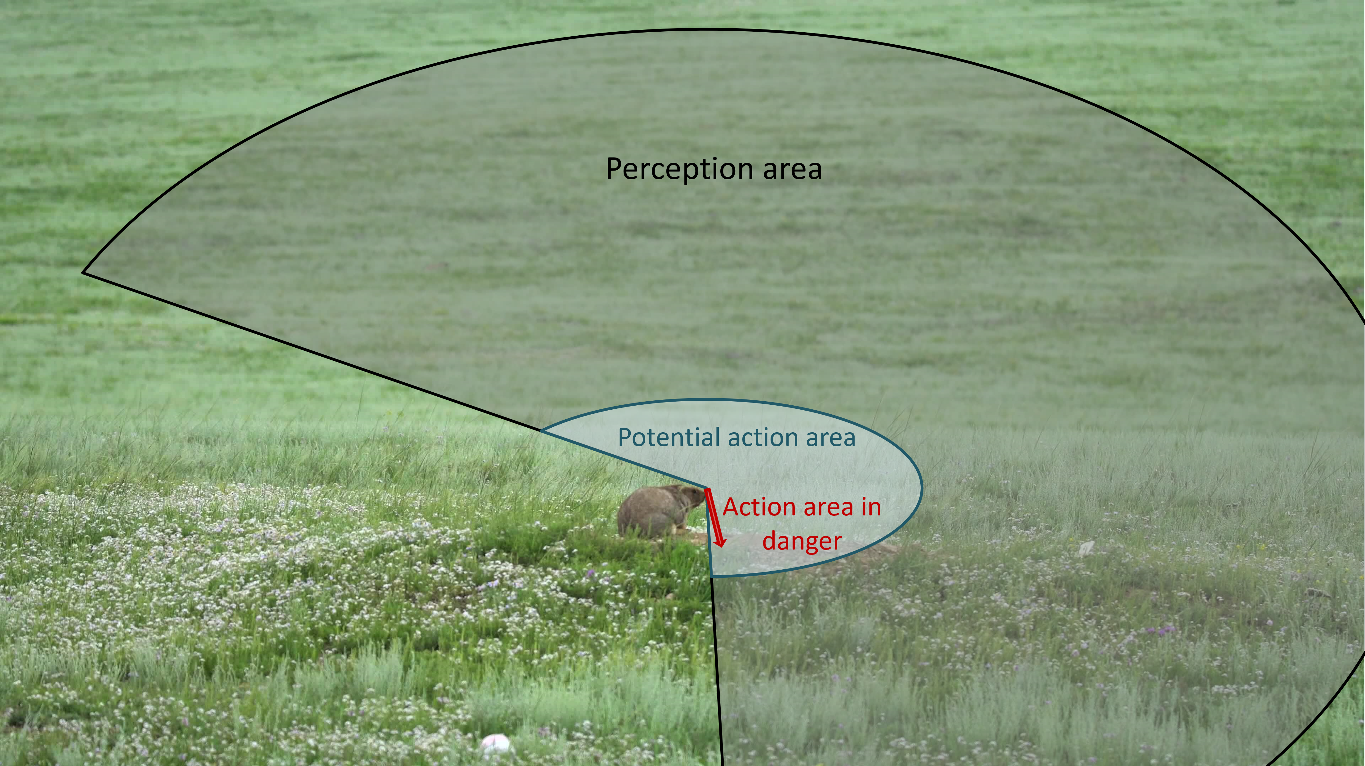
Figure 9.6: This marmot looks out for predators within a large perception neighbourhood. If it does not sense a predator, the potential area to which it can physically move in the next time step is the action area. In case of danger, the action area is narrowed down to a straight line into its cavity.
Exercise: GAMA model to represent perception and action neighbourhoods
Add action neighbourhoods to the GAMA perception neighbourhood model of the previous GAMA exercise in this lesson. Let both, the angle and the size of the action neighbourhood be smaller than the parameters for the perception neighbourhood.
No additional features are used to implement action neighbourhoods. So you should be able to code the model yourself. If you need support, view the code below, or post a question into the discussion forum.
View the model code.
model Ex_L7b_perception_action_neighbourhood

global {
    // the radius and angle of the perception neighbourhood
    float vision <- 7.0;
    float vision_angle <- 120.0;

    // the radius and angle of the action neighbourhood
    float step_length <- 3.0;
    float action_angle <- 45.0;
    init {
        create ants_circle number: 1;
        create ants_arc number: 1;
    }
}

species ants_circle skills: [moving] {
    list<point> trajectory <- [];

    reflex ant_move {
        // random walk
        do wander speed: step_length;
        add location to: trajectory;
    }

    aspect ant {
        draw circle(1) color: #black;
        draw line(trajectory) color: #black;
    }
    aspect perception {
        draw circle(vision) color: #grey;
    }
    aspect action_neighbourhood {
        draw circle(step_length) color: #magenta;
    }
}

species ants_arc skills: [moving] {
    list<point> trajectory <- [];

    reflex ant_move {
        // correlated random walk
        do wander amplitude: action_angle speed: step_length;
        add location to: trajectory;
    }

    aspect ant {
        draw circle(1) color: #green;
        draw line(trajectory) color: #green;
    }
    aspect perception {
        // draw an arc with the diameter (the GAMA documentation says "radius", but it needs to be the diameter), the heading and the width of the vision's angle.
        draw arc(2*vision, heading, vision_angle) color: #limegreen ;
    }
    aspect action_neighbourhood {
        // draw an arc with the diameter (the GAMA documentation says "radius", but it needs to be the diameter), the heading and the width of the action angle.
        draw arc(2*step_length, heading, action_angle) color: #magenta ;
    }
}

experiment simulate type: gui {
    output {
        display map {
            species ants_circle aspect: perception transparency:0.1;
            species ants_arc aspect: perception transparency:0.1;
            species ants_circle aspect: action_neighbourhood transparency:0.1;
            species ants_arc aspect: action_neighbourhood transparency:0.1;
            species ants_circle aspect: ant;
            species ants_arc aspect: ant;
        }
    }
}
9.4.5 Interaction
A special - and important! - case of action is, when an agent triggers or responds to a dynamic change in the environment or when two agents act on and therby adapt to each other.
The implementation of dynamic interaction between agents or agents and cells is a bit trickier than defining the behaviour of individual agents. Interaction between two agents (or agents and the CA) requires the overlay of agent locations with perception areas and action areas that define a subset of agents (or cells) for which the interaction is triggered. We will look into socially adaptive behaviour by the example of movement of smart entities, in the next lesson.