UNIGIS module: Spatial Simulation
19 May, 2026
Lesson 1 Spatial Simulation: an overview
Preface
This web-book is a text book with exercises that together form the learning materials for “Spatial Simulation”, an elective module of the UNIGIS distance learning program in Geoinformatics at the University of Salzburg.

The web-book is published under an open licence. I welcome everybody to explore the contents and to work through the simulation modelling exercises. Only the related discussion forum and the assignments can exclusively be accessed by actively enrolled UNIGIS students, who signed up for this module.
About this web-book
Spatial simulation integrates the dimensions of space and time and thus explicitly represent process dynamics in its spatial context. This includes a wide range of application areas, such as transportation, hydrology, population ecology, healthcare, land-use change, wildfire prevention, etc. Depending on the nature of a specific spatio-temporal phenomenon, a multitude of methodological approaches have been developed. The wide range of model categories is confusing at the first sight: there are mathematical, numerical, analytic, probabilistic, stochastic, deterministic and individual-based models.
In the first part, this module provides a theory-based categorisation of models and the respective type of problems they can solve. You will gain the competence to identify the most adequate modelling approach for your research interest or problem domain. In the second (main) part, there will be a specific focus on models that explicitly incorporate the spatial perspective in their structure: cellular automata and agent-based models.
For exercises and assignments, the open-source modelling framework ‘GAMA’ will be used. The programming language GAMA was explicitly designed for coding agent-based models. This modelling platform is particularly well suited to work with GIS data. It comes with a great wealth of model examples that are openly accessible and usable through GAMAs model library. From there, you will learn to use, modify and design your own models and how to use your own GIS data.
For me, it was a great experience to design and write this module. My own motivation to take this effort was rooted in the experience that I made, when I was a PhD fresher, desperately looking for a textbook that would help me getting an overview over a confusing variety of spatially explicit modelling methods. I hope, this module helps to fill the gap.
One last request: This is a living document. I try to provide and maintain high-quality and up-to-date materials. Please report any issue that you may find to the UNIGIS issue tracker on GitHub (account needed) or drop me an email.
kind regards Gudrun Wallentin
This web-book is licensed under a Creative Commons Attribution-NonCommercial-ShareAlike 4.0 International License.

1.1 Models
This first lesson sets the frame for this module. It looks into the concepts of models and systems, discusses alternative purposes for modelling, and reviews typical application areas. On the more practical side, the GAMA modelling platform is introduced with a first, “Hello World” exercise.
Upon completion of this lesson, you are able to…
- understand the nature of systems and the purpose of simulation modelling,
- decide, whether or not a particular problem can be addressed with spatial simulation modelling,
- use the GAMA simulation platform for a “Hello World” model.
Everything we think we know about the world is a model (Meadows and Wright 2008)
This is a rather philosophical way to think about models. In Geoinformatics, models are part of our daily work. The same real world phenomenon can be represented in different ways, e.g. as raster or as vector models. An architect may work with physical models, e.g. mini-buildings made of paper to visualise his ideas to the public in a tangible way. Although simplified, such paper house needs to be sufficiently detailed to enable neighbours to envision the future building.
The commonly accepted definition for models is the following:
Models are abstract and simplified representations of reality that are designed for a particular purpose.
Following up this definition, simulation models are computer models that iteratively recalculate the state of a system as it changes over time, where the recalculation is based on mathematical, empirical and / or logical relationships that describe the system (O’Sullivan and Perry 2013).
In this module we talk about spatial simulation models, which represent both, space and time in an integrated way. The terms ‘spatio-temporal models’ or ‘dynamic models’ are therefore often used synonymously for spatial simulation models.
1.2 Areas of Application
Simulation modelling can be used in a wide range of application domains, including
- Environmental planning
- Climate change impact and mitigation planning
- Manufacturing applications
- Construction engineering
- Military applications
- Logistics, transportation, and distribution applications
- Business process simulation
- Healthcare
The common denominator of all application domains listed above is that we can model, analyse and visualise complex systems. In the early times of simulation modelling, where computer power was limited, modellers were restricted to abstract and generic models. This provided new and insightful views on the general functioning of studied systems, but hardly could be applied to specific study areas. Only since the advent of strong and fast computers, it has become possible to model real world systems and accordingly explore real world problems across space and time.
The video below (Figure 1.1) is provided by the developer team of the GAMA modelling software, which we will use in this module. There you will see, how GAMA earns its reputation to be the best agent-based simulation modelling software for dealing with large scale GIS data. The video shows some quite impressive real world application examples. There comes no audio information with it. Thus, you can just switch off the rather annoying background sound, if you want.
Figure 1.1: An introduction to the main functionality of GAMA modelling, demonstrated with some impressive application examples. 4:30 min
Simulation modelling is not a trivial task and it clearly is on the advanced side of the spatial analysis toolbox. Despite a much increased usability of simulation modelling frameworks, it takes quite some expertise to adequately design, implement and validate a model such way that it is useful to solve a problem. Before we start to think about HOW to solve problems with simulation models, we take our time to think WHY we want to use simulation models. Or to phrase it differently: for which problems should we use simulation models and for which problems can (and should) we use simpler approaches?
The short answer to this question: simulation models are appropriate for problems that cannot - or only at great expense - be studied in the real system or a physical lab experiment. This might be the case, if the studied system.
- is dangerous, e.g. explosions of nuclear power plants,
- is large, e.g. questions related to global climate change,
- has a time scale that exceeds reasonable time frames of physical experiments, e.g. geological plate tectonics,
- is unethical, e.g. scenario testing for the spread of diseases,
- is a historical system in the past, e.g. expansion of the Roman Empire.
- manipulations of interest would impact the system in inadequate ways, e.g. forest fire distribution with respect to different management regimes,
- involves a significant portion of randomness and we want to learn about the range of potential system behaviour (process variability).

Figure 1.2: Simulation models are sophisticated tools. Although, they can be very helpful, it is not appropriate to use them for simple tasks.
If a problem can be solved by common sense or analytically, the use of simulation is unnecessary. Additionally, using algorithms and mathematical equations may be faster and less expensive than simulation modelling. Also, if the problem can be solved by performing direct experiments on the system to be evaluated, then conducting direct experiments may be more desirable than simulating.
In summary, simulation models are appropriate to solve complex problems. Specifically, if:
- the problem cannot be solved using common sense,
- the problem cannot be solved analytically,
- real-world experiments cannot be performed, because they would be too big, dangerous or costly,
- the time and resources to build a model are available,
- there is a basic understanding of the system of interest,
- it is possible to validate the model.
1.3 Complex systems
Weaver (1948) offered an interesting view on complexity. He argued that classical science traditionally has focused on systems with either just a few or a great number of elements. In the first case problems can be solved analytically (i.e. with mathematical equations), latter problems can be treated with statistical methods. Unfortunately, in the real world we often find ‘middle-numbered’ systems between these two extremes with too many unknown variables for an analytical solution and at the same time not enough to average out. Single events in such complex systems can have large impact on the results and outcomes are hard to predict.
Along these lines, decision making situations can be categorised into four problem domains that afford different solution strategies - known as the ‘Cynefin (kʌnɨvɪn) framework’ (Snowden 2000):
Simple problems can be solved by straightforward categorisation; there is a clear ‘best practice’ solution
Complicated problems need to be analysed to find an adequate solution. The solution represents ‘good practice’ (there might be other good solution too)
Complex systems follow some guiding principles, but the behaviour of the system cannot be intuitively predicted: it ‘emerges’ from the behaviour of system components. This problem domain lends itself for simulation modelling as tool that helps solving problems.
Chaotic systems have no inherent causal relationships, every situation is novel and the first solution strategy is immediate action to stabilise the system.
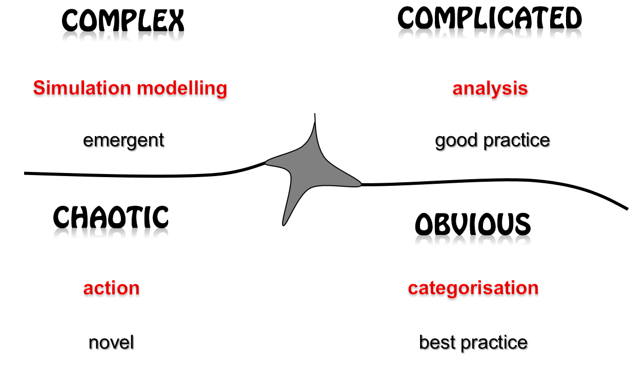
Figure 1.3: Cynefin framework
Before we dive deeper into modelling, Table 1.1 provides a definition of some important terms:
| Term | Definition |
|---|---|
| Conceptual models | break down a real world phenomenon into parts that are relevant for the model’s purpose. |
| Physical models | are ‘hardware’ models, such as wind tunnels to investigates the airflow around the downscaled replica of a wing of a plane. |
| Simulation models | are computer models to conduct virtual experiments, and to find out how the system behaves across space and time. |
| Theoretical models | describe relations between its components rooted in theoretical considerations in the literature. |
| Mathematical models | describe the relation between system components with help of mathematical equations |
| Analytical models | are models that can be solved exactly with pencil and paper by using mathematical reasoning. |
| Numerical models | are mathematical models that cannot be solved exactly. They slice continuous space / time into discrete pieces for a stepwise approximation. |
| Empirical models | describe the relation between system components by observational evidence. |
| Deterministic models | are fully reproducible: the same parameter settings lead to the same outcomes. |
| Stochastic models | have random elements encoded. Outcomes thus vary between model runs. |
1.4 Why do we need simulation models?
1.4.1 Prediction
What will the future look like? Arguably, this is one of the most tempting questions that we have, when somebody presents a simulation model to us. This is natural human curiosity and after all, it has been accurate predictions that pushed forward scientific knowledge and our understanding of the world. The position of stars can be exactly predicted based on the understanding of planetary orbits, and chemical reactions are explained by our understanding of atoms and molecules.
The purpose of simulation models traditionally was to predict the future state of a system. Systems that we understand very well and for which we have abundant, reliable and detailed data are the ones that are most suitable for prediction modelling. Typical application domains for predictive models are traffic, hydrology, or evacuation management.
Unfortunately, simulation models do not lend themselves for accurate predictions. Other than for problems that can be solved analytically (as for engineered systems) or probabilistically (as for weather), simulation models target at the study of the very nature of a complex, living system. Thus, simulations always have a range of uncertainty associated with them. Weather forecasts are prominent examples for the prediction of stochastic (random) processes: meteorologist can predict tomorrow’s weather, but we never can be completely sure that the forecast will be correct. Often the meteorologist therefore uses phrases like: “the probability of rain showers are highest in the west” or “in the afternoon or early evening, first snowfall is expected”. These statements express spatial, temporal and attribute uncertainties.
For some problems, we might have tons of data, but still we do not thoroughly understand the underlying processes. Global financial markets are an example for such systems. Modelling in this case can help in the development of theories.
Other problem areas revolve around questions that are well routed in underlying theoretic understanding, but are lacking detailed data. Population dynamics of most animal groups are a good example, here.
Last but not least, we have these nasty questions where we cannot draw on many data, nor on good process understanding of the studied phenomenon. The most adequate use of simulation models in such cases is to use models as ‘tools to think with’, i.e. learning devices that help the researcher in gaining a better understanding of the system and also guide towards the areas with most pressing need for data.
1.4.2 Models to guide data collection
For simulation models that are explicitly defined to solve a real world problem, it is essential to have reliable real-world data. The primary role of a simulation model in this case is to assess the sensitivity of model predictions to changes in the input parameters. This way, it is possible to determine the most critical empirical data that are needed to improve our understanding of the system. This kind of analysis is called ‘sensitivity analysis’ and it involves a systematic change of input parameters to find out which parameters have the strongest effects on the system behaviour.
An example for an application domain that frequently takes advantage of simulation models to guide data collection are conservation efforts of endangered species. On the other side, a rather depressing evidence of a misuse of simulation models is the case of fisheries in the Adriatic Sea: not least because of the ignorance of uncertainties in input parameters, stochastic behaviour of the system led to policies that resulted in overfished ecosystems.
Data shortage has been a great issue in the past and it still is in certain application fields and certain areas of the world. However, as we collect information continuously in automated ways the situation has changed fundamentally. Consequently, we are in the situation to have huge amounts of empirical data, but we are still lacking clear understanding of causal relationships that govern the dynamics of the underlying system. Simulation models can help to close this gap.
With the help of simulation models we can test various hypotheses against data and thus gain increasing understanding of the system. The major problem of this approach is the equifinality problem, which refers to the problem that there might be several models that equally well describe the state of a system. We thus might be misled, if we assume that a simulation outcome that reproduces the state of a real system results from a correct model. Later in this module we will discuss a way to address this problem of equifinality with the approach of ‘pattern oriented modelling’ (Grimm et al. 2005).
1.4.3 Simulation models in science
In scientific research, simulation models are increasingly used as heuristic learning tools to gain a better understanding of a particular system. As such spatial simulation models are a relatively recent addition to the scientific toolbox, that can be thought of ‘virtual laboratories’ for hypothesis testing. This is an essential part of research in the hypothetico-deductive approach – the standard approach to acquiring new knowledge in (natural) sciences
The hypothetico-deductive approach in science
- Formulate a hypothesis
- Deduce predictions from the hypothesis for a specific problem in a specific study area
- Test the prediction in an experiment
- Analyse the results: does the hypothesis hold or was it falsified?
Taken that simulation models in this context can be conceptualised as laboratories, simulations conform to experiments to test a hypothesis. Just as in ‘real’ experiments, the status of the system is recorded and tracked throughout time for subsequent analysis.
1.5 How to solve problems with modelling
1.5.1 Definition of the purpose
The nature of the problem that needs to be solved determines the purpose of the model. In scientific models the hypothesis equals the problem. There is no model for the sake of its own and every model is developed for a particular purpose. Or to put it the other way round: every problem needs its own model. Clearly, some parts of one model can be used for another model with a similar purpose. However, there is nothing like a ‘generic’ model, nor a model that is generally ‘valid’. The purpose guides the modeller on how to break down the real world system under investigation to a conceptual model. Further, it is the model’s purpose that helps to select an adequate modelling approach.
Therefore, the ‘problem definition’ is the first step for the development of any model. It needs to be an explicit, specific and operational definition of the problem at hand. Usually is stated as hypothesis or as product specification.
1.5.2 Conceptual model
Let’s consider a real world phenomenon that we want to study to solve a related problem. For example, a delegate of the European Union, who wants to know about the impact of alternatively discussed agricultural subsidy regimes on land use change across Europe. Or a bank director, who wonders whether he should invest in a ski resort in the Swiss Alps, despite climate change.
The first step in model development is to design a conceptual model. To do so, we need to explicitly define purpose, scope, grain and extent of our model. Further, the phenomenon under study is broken down into general elements:
System components are discrete entities that represent the elements of the system under study, which are relevant to the model’s purpose, e.g. tourists from different destinations across Europe.
State variables are attributes at system level or at the level of particular components that allow for quantitative measurement of the state of a system, e.g. annual revenue in Swiss ski resorts.
Interactions describe, which system components are interrelated and how these relationships are organised, e.g. word of mouth effect between tourists from the same destination about recent snow cover.
Processes describe, how a system and / or its components evolve over time. Depending on the modelling approach, processes might be described theoretically (rule-based models), statistically (empirical models), or mathematically (system dynamic models), e.g. the linear increase of temperature in the Swiss Alps over the next 50 years.
1.5.3 Choosing a modelling approach
Simulation models can conceptualise the system from a top-down (system-level) or a bottom-up (individual-level) perspective. In this module we will focus on bottom-up modelling approaches, as they disaggregated down to the level of individual entities and thus are more relevant for solving spatial problems. For now, there is a brief description of core characteristics of the three main approaches to simulation modelling:
System Dynamics models describe relations between sub-systems (components) with help of differential equations. Components are aggregated and quantifiable entities, e.g. populations, biomass, market stocks or the volume of water in a lake. System Dynamics models are deterministic, continuous over time, and inherently non-spatial.
Cellular Automata models describe relations between neighbouring cells in a grid for each time step with help of if-then rules. These models can be deterministic or stochastic, depending whether randomness is incorporated in the rules; they are discrete in time and inherently spatial.
Agent-based models describe local relations between individual objects (=agents) and their local environment based on a set of rules. Agent-based models are stochastic, discrete in time and inherently spatial.
1.6 GAMA modelling software
GAMA stands for “GIS and Agent-based Modelling Architecture”. It is a modelling environment to develop spatially explicit simulation models. In this module, the latest stable version of GAMA is used to code Geosimulation models. Please follow GAMA’s installation guidelines to download and install the software on your machine.
GAMA resources
GAMA Platform provides a collection of resources (tutorials, documentation, …) in the latest version of GAMA code. In this module, there are exercises that should equip you with all the necessary skills to manage the assignments. However, of course you are always welcome to explore further!
Watch the official “Hello World” instruction to GAMA provided by the GAMA developers (Video 1.4) to get a 10-min intro to the GAMA platform. The tutorial is quite comprehensive - don’t expect to follow in the speed in that the platform and the model is presented. However, once you have the model successfully implemented, you are ready for the first exercise, where you will implement your own Hello World model in GAMA.
Figure 1.4: Video 9:40min. Tutorial to get started with GAMA.
At the end of this lesson, there are two “Hello World” exercise that will introduce you modelling ABM and CA with GAMA.
Exercise: Hello World ABM
In this Hello World exercise you will put into practice, what you’ve seen in Video 1.4. You will build a simple and abstract model of a system in the African Savannah. It consists of the following entities:
- 20 lions that walk around randomly. A lion is visualised as an orange circle with the size of 3.
- 20 zebras that also walk around randomly. A zebra is visualised as a grey triangle with the size of 2.
Every time, when a lions randomly runs into a zebra, it kills the zebra. The behaviour of killing a zebra is modelled in a “reflex” procedure of a lion.
GAMA is a very polite language. So if one agent wants anything from another agent, it will ask the other agent to do something. In this case, to make lions kill zebras, the attacking lion asks the nearby zebra to “do die”:
ask zebras at_distance 2 {
  do die;
}
While coding, always make sure that you set the indents correctly. If GAMA highlights an error (red) or a warning (yellow), hover over the error and read the error message. Try to understand, what went wrong in order to be able to fix it. Once you are done, run the experiment to check, whether everything works like expected. If there are still errors, GAMA will not run the experiment. Warnings are ignored, but try to fix them anyways.
Now, try to implement the model in GAMA. If you get stuck, you can look into the code of the worked solution below. However, there’s more than one way to skin a cat. The code solutions that I provide for the exercises in this module are just one way of doing it. As long as it works, everything is fine - at least for now. Only, if dealing with large, geographic data sets, the modeller needs to think about computational efficiency of the code.
See model code!
/**
* Name: Ex L1a - Hello World
* Author: WALLENTIN, Gudrun
* Description: Exercise of the UNIGIS Salzburg optional module
* Hello World agent-based model
*/

model ExL1a_HelloWorld

global {
    init {
        create lions number:20;
        create zebras number:20;
    }
}

//lion agents
species lions skills:[moving] {
    reflex move {
        do wander ;
    }

    reflex attack when: !empty(zebras at_distance 2) {
        ask zebras at_distance 2 {
            do die;
        }
    }

    //visualisation settings for lions
    aspect base {
    draw circle(3) color: #orange ;
    }
}

//zebra agents
species zebras skills:[moving] {
    reflex move {
        do wander;
    }

    //visualisation settings for zebras
    aspect base {
    draw triangle(2) color: #grey ;
    }
}

//Simulation
experiment main_experiment type:gui {
    output {
        display map  {
        species lions aspect:base;
        species zebras aspect:base;
        }
    }
}
Enough of lions and zebras! For now, you have gained enough understanding of how to represent smart agents in a GAMA model. Let’s move to the second “Hello World” model, which will look into the representation of a dynamic environment in GAMA with the Cellular Automaton approach.
Exercise: Hello World CA
This exercises introduces into how to define and implement Cellular Automata in GAMA.
Create a CA
GAMA handles a grid of cells similar to a set of agents. While agents are called “species” in GAMA, a CA is called “grid”. Each cell in a grid has built-in variables and the possibility to define further custom variable. To keep your model in order, always put the grid after the species sections, as the last section before the experiment.
Let’s create a CA with 10 by 10 cells:
model ExCellularAutomata

global{
}

grid myCA width: 10 height:10 neighbors:4 {
}

experiment simulation {
}
As you can see in the grid parameterisation, this creates a raster in which each cell is aware of its 4-neighbours (van Neumann neighbourhood). The statement neighbors:8 results in a 8-neighbour Moore neighbourhood, and neighbors:6 will create a hexgrid.
Next, we need to display the cells in the output. This is done in the experiment section. There we define that we would like to have a map display that visualises the grid “myCA”. The border of individual cells can be visualised by adding the border facet to the grid in the experiment section: grid myCA border: #gray;, like it is displayed in Figure 1.5. However, once the grid is not empty, the visual experience is usually nicer without borders.
// Define an experiment that visualises the CA
experiment simulation type: gui{
    output{
        display myMap{
            grid myCA border: #gray;
        }
    }
}
When you start the simulation now, you should be able to see the CA. It should be looking like Figure 1.5.
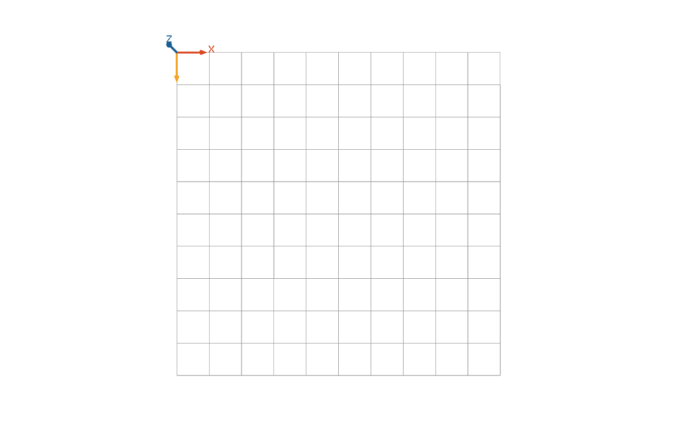
Figure 1.5: An empty cellular automaton in the map display of the simulation.
Next, explore what happens, when you change the neighbourhood. Change the parameter neighbors to 6 or 8 and look at the results.
Declare and assign variables
Variables are always declared at the beginning of the section, to which they belong: global variables at the beginning of the global section, agent variables at the beginning of its species section and CA variables at the beginning of the grid section. The declaration of a variable consist of the definition of the data type followed by the variable name:
grid myCA width: 10 height:10 neighbors:4 {
  int elevation;
}
This CA now has a variable called elevation that is of type integer (i.e. whole numbers, without digits after the comma). As elevation is defined as a grid variable, each single cell can have a different value and we can represent an entire DEM with this variable.
After the declaration, you can assign a value to that variable. If you want to assign a value only once in the beginning, you can assign the value together with the declaration. The below code will return a grid with an elevation value of type float that varies randomly over the CA between 0 and 255.
grid myCA width: 10 height:10 neighbors:4 {
  // declare the elevation variable of type float and assign a random value between 0 and 255 to it
  float elevation <- rnd(255.0);
}
Don’t be disappointed, if the elevation variable is not visible in the simulation output myMap. To visualise it, we can make use of the built-in grid variable color and visualise the grid in the experiment.
Built-in variables
“Built-in” means that this variable is predefined and a GAMA modeller can use it without declaring it. Every cellular automaton in GAMA (i.e. a grid) has the following built-in variables:
- grid_x contains the column index of a cell.
- grid_y contains the row index of a cell.
- color is of type rgb and holds the 3 integer values between 0 and 255 that are needed to define a colour.
- neighbors is a list of the 4, 6 or 8 neihgbouring cells.
- grid_value is of type float and holds the value for each cell.
Use color to visualise variables
Let’s visualise the elevation with a gradient of red colours. The rgb values of the built-in variable color span from 0 to 255. If you let one colour be a variable, you can see visually, how the variable changes throughout the simulation. Just assign the elevation variable as the red component of color variable of the grid to display the elevation variable along a red gradient:
grid myCA width: 10 height:10 neighbors:4 {
    // declare the elevation variable of type float and assign a random value between 0 and 255
    float elevation <- rnd(255.0);
    //define the 8-bit colour shades for red, green and blue with values between 0 and 255.
    rgb color <- rgb([int(elevation),0,0]);
}
Run the experiment. Does the result look anything similar to Figure 1.6?
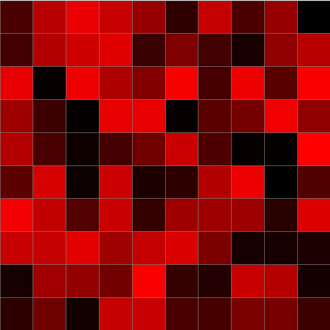
Figure 1.6: Result of a random colour assignment in the initialisation of the grid species.
See the code to double-check
/**
* Name: Ex L1b - Hello World CA
* Author: WALLENTIN, Gudrun
* Description: Exercise of the UNIGIS Salzburg optional module
* Hello World Cellular automaton model
*/

model ExL1b_HelloWorldCA

global{
}

grid myCA width: 10 height:10 neighbors:4 {
    // declare the elevation variable of type float and assign a random value between 0 and 255 to it
    float elevation <- rnd(255.0);
    //define the 8-bit colour shades for red, green and blue with values between 0 and 255.
    rgb color <- rgb([int(elevation),0,0]);
}

// Define an experiment that visualises the CA
experiment simulation type: gui{
    output{
        display myMap{
            //borders are optional and usually omitted: they don't look pretty in continuous environments
            grid myCA border: #gray;
        }
    }
}