Lesson 7 Dynamic environments
Environments in complex systems are dynamic. Evolution and change at the landscape level emerges from processes at the local scale: urban sprawl emerges from settlers who build their houses, erosion emerges from water drops that run down a slope, and the range expansion of invasive species emerges from seed dispersal and germination. Looking at dynamic environmental phenomena at a highly abstract level, we can state that they fall under just four process categories (see also O’Sullivan and Perry 2013): 1) global or regional trends, 2) growth (including spread and diffusion), 3) aggregation (including segregation), and 4) movement. This lesson introduces into the local processes, which mechanistically describe the emergence of dynamic phenomena at landscape level. With just a handful of CA building block models (or a combination thereof) that implement these local processes we can model environmental dynamics of complex systems.
Upon completion of this lesson you will be able to ..
- identify local process types that are underlying the change dynamics of landscapes,
- implement typical local processes in a cellular automaton (‘building block models’),
- apply and combine building block models to mechanistically represent the emergence of more complex environmental dynamics.
7.1 Global trends
The state of the environment can change over time. From a modelling perspective, global trends are non-spatial attribute changes that are equally applied to each cell of a cellular automaton CA without taking into account the state of neighbouring cells.
Typical examples for global trends are temperature increase due to climate change, forest biomass regrowth after logging, or seasonal oscillations of CO2 concentrations.
A state change can be discrete (disruptive), but more commonly it is a continuous growth or decay process. Analogous to system dynamics modelling, continuous change is implemented as stepwise approximation of difference equations that represent linear, exponential or logistic growth or decay. For a quick recap on the mathematical expression, refer back to the Chapter Growth and decay in the lesson on System Dynamics.
In Figure 7.1 the respective growth and decay difference equations are coded into a cellular automaton model to serve as the building block model for global trends, implemented with NetLogo.
A special case applies, if the parameters of the state change vary over space. For example, if the carrying capacity increases, the further south the cell is located. This case results in spatial environmental gradients that may grow or shrink over time (which is not implemented here).
Figure 7.1: Global trends: linear, exponential and logistic growth & decay - building block CA models, implemented in Netlogo.
For further reference, you can download the GAMA building block model “global trends”.
7.2 Growth processes
7.2.1 Eden growth
Growth describes the expansion of something into adjacent regions. The basic way to model growth was suggested by Eden (1961). Therefore, growth models are often addressed as ‘Eden growth models’. The rules of the basic approach are simple:
- Seed an initial site and occupy it
- Randomly select an unoccupied neighbour
- Occupy this neighbour
Looking at these rules a bit closer, you will realise that this corresponds to the “stochastic CA” model that we have discussed in depth in the previous lesson. The emergent pattern of this modelled process shows a compact and dense interior with a diffuse and fringed edge (the actively growing zone). This pattern strongly reminds of growing bacteria, lichen or cities (Figure 7.2).
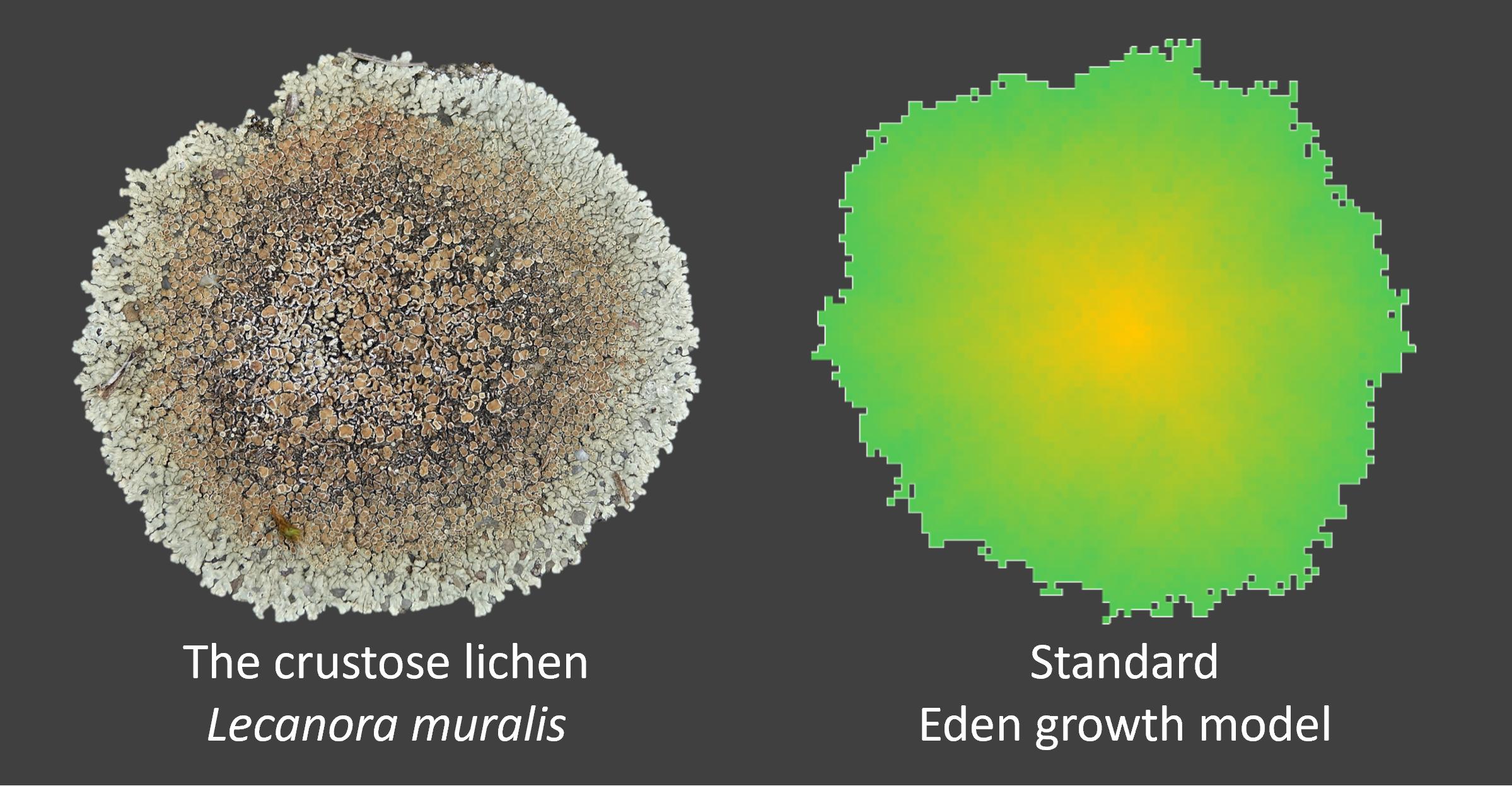
Figure 7.2: Models that simulate biological growth are named after Murray Eden, who first formally described this process.
For further reference, you can download the GAMA building block model “Eden growth”.
7.2.2 Percolation
Percolation describes the expansion processes through a porous material. In a wider sense, any process that operates on a heterogeneous (“porous”) surface can be modelled as a percolation process. For example, the spread of a disease through a population, the spread of a wild-fire through a sparse forest, groundwater movement through the aquifer, or population expansion in fragmented landscapes.
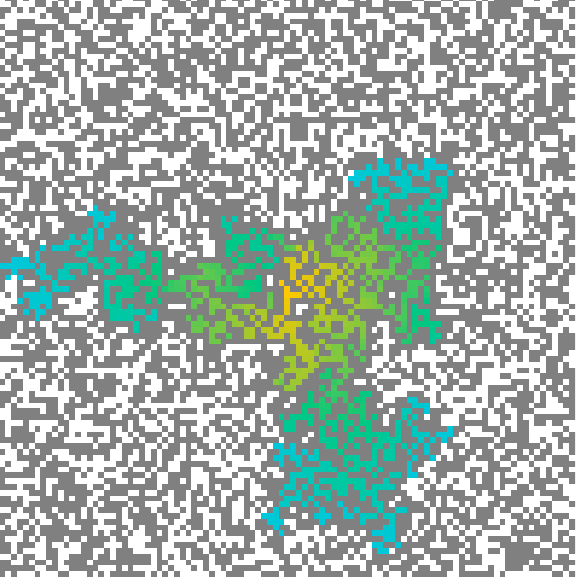
Figure 7.3: Percolation models simulate the expansion of something in porous matrices.
In simulation modelling, the representation of the ‘porous’ background of a percolation model can be modelled by a grid with loosely occupied cells, or alternatively as linked cells or graphs. According to percolation theory, the porosity is critical to the expansion process. If it is too sparse, percolation will stop after very few steps. If it is too dense, the entire study area will be percolated. The phase transitions at which percolation behaviour change between too sparsely, optimal and too densely occupied grids are sharp.
Exercise: Percolation - porosity dependence
You have already encountered the NetLogo wildfire model to explore neighbourhood effects (Figure 6.3). In this exercise, we work with the original wildfire model from the NetLogo Library to focus on the dependence of model outcomes on the “porosity” of the background matrix (Figure 7.4).
Green cells represent trees in a sparse forest, black cells are not covered by trees. The fire starts from the left side and percolates through the forest until no further trees are close enough to be ignited. Can you find the critical forest density value above which the fire affects the entire forest?
See solution!
The critical value (for the particular wind conditions) lies around 59%: at this value, there is a 50% chance that the fire reaches the other side of the forest. This probability sharply drops for a forest density that is only slightly reduced, whereas the entire area gets burned in slightly denser forests.
Figure 7.4: Explore, the impact of forest density on the spread of a wildfire, NetLogo Web
For further reference, you can download the GAMA building block model “Percolation”.
7.2.3 Spread
Spread describes processes of spatial expansion to other regions that are usually close, but do not necessarily have to be adjacent.
A spread model is based on the Eden growth model. However, the neighbourhood definition includes sporadic jumps to represent long distance dispersal events. Jump events are rare, but they greatly contribute to rapid expansion in spread processes. The emergent pattern exhibit the typical disjunct distribution “islands” (Figure 7.5).
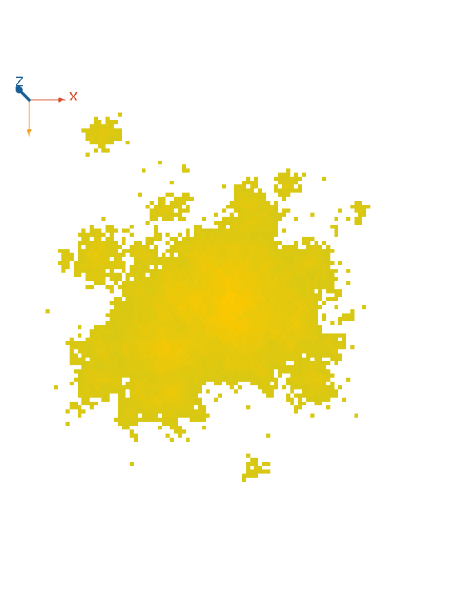
Figure 7.5: Spread models simulate the expansion like Eden growth models, but they are not bound to adjacent neighbours and include occasional long distance dispersal events.
A commonly encountered example for spread processes is the habitat expansion of invasive species, where select individuals are distributed through human activity, e.g. along highways. In Figure 7.6, you can see a typical spread pattern by the example of an invasive fly in the United States.
Figure 7.6: The spread process of the invasive spotted-wing drosophila fly in the US exhibts jump dispersal. Click on the figure to start the animation. Animation source: Dispersal.jl
On the algorithmic side, jump dispersal is modelled with an inverse distance probability function. The farther a cell is from an invaded cell, the smaller the chance it will get invaded itself.
For further reference, you can download the GAMA building block model “Spread”.
7.2.4 Diffusion
Diffusion describes the movement of material from regions of high concentration to regions of low concentration. Diffusion has very similar geometric properties like growth. The main difference is that in diffusion processes attribute values get diluted over time, whereas the nature of the growing object stays the same.
Let’s consider how diffusion processes operate: particles that are suspended in a fluid, or in the air move around randomly. This surprising behaviour was first described by Robert Brown in 1827 and 80 years later explained by Einstein, who correctly claimed that this movement is due to collisions with water molecules. It served as evidence of the existence of molecules. Random movement is thus also called “Brownian motion”.
Following from Brownian motion, particles do not actually move from high to low concentrations: they all move anywhere into all directions. However, there are more particles in high concentration regions so that in the end there is a net effect of diffusion from high to low concentrations.
The commonly applied algorithm to capture the diffusion process is the application of a moving window kernel that computes the mean of each cell’s neighbourhood, including the cell itself. Figure 7.7 demonstrates the simplest case of a uniform diffusion in a Moore neighbourhood. All values in the kernel are summed up and then devided by 9. The same method is also used as “low pass filter” in image processing for smoothing or noise reduction.
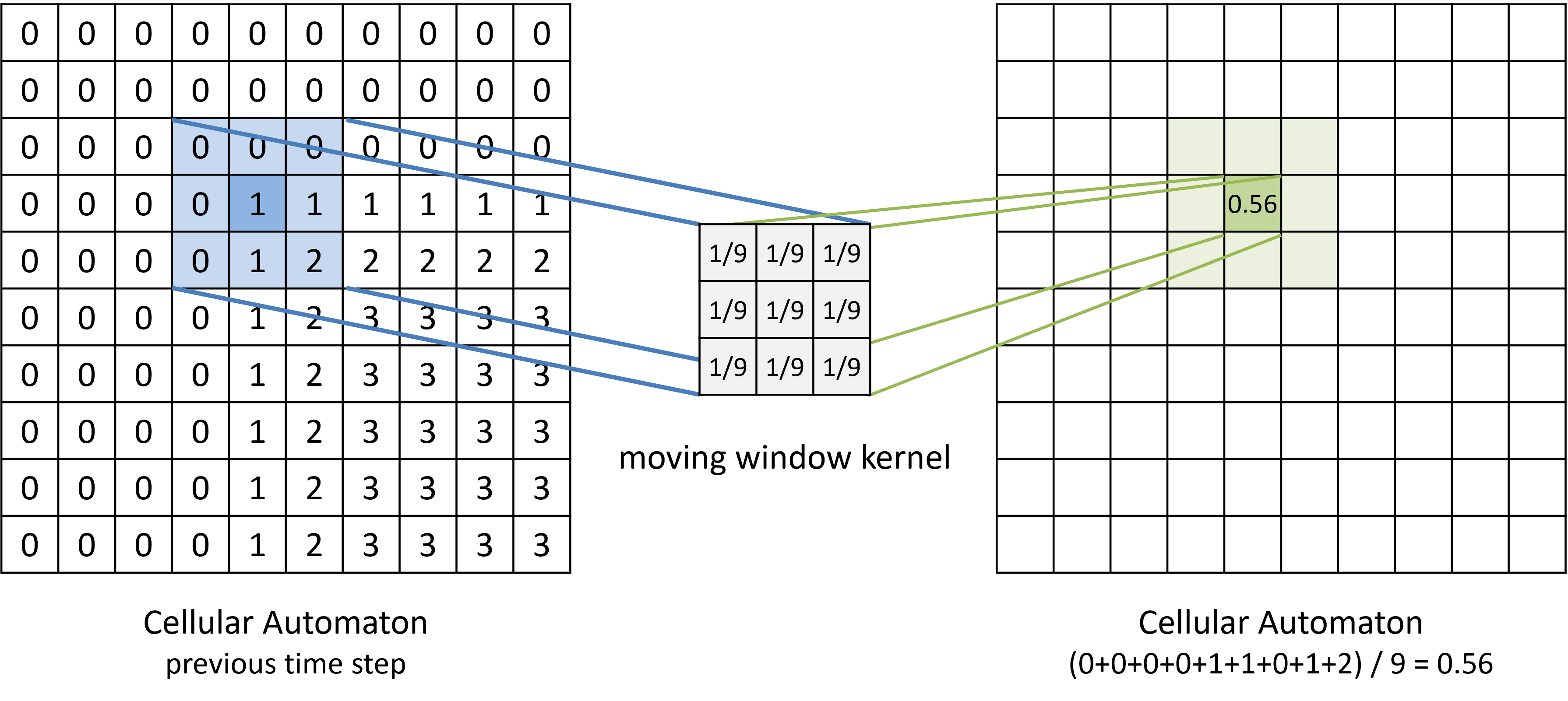
Figure 7.7: Moving average kernels model diffusion processes in cellular automata.
Common CA modelling platforms like GAMA and NetLogo offer built-in methods that implement diffusion. For Hungry Minds, please refer to the GAMA documentation on diffusion to explore the details and parameters for diffusion modelling that are offered by GAMA.
For further reference, you can download the GAMA building block model “Diffusion”.
7.3 Aggregation
Aggregation and segregation are closely related processes. Whereas aggregation refers to the process of spatial clustering of one type of entity, segregation refers to the process in which different types of entities separate. If the initial distribution of two populations is randomly distributed in space, then the aggregation of one entity will entail a segregation process: more related things tend to cluster together, which leads to a segregation of dissimilar things. The result of such processes is a heterogeneous, non-random and clustered (=patchy) world.
7.3.1 Schelling’s segregation model
Thomas Schelling’s models of spatial segregation of people with different nationalities in a city (Schelling 1971) are among the most famous spatial simulation models. Cells may take three states: vacant, blue and red. The two coloured cells tolerate cells of opposite colour in their neighbourhood, but desire to be surrounded by a minimum proportion of cells of the same colour. If a cell is ‘dissatisfied’ with its current location, it can switch to the closest ‘vacant’ location with a satisfying neighbourhood. Cells are ‘relocated’ until the desired neighbourhood is reached for all cells, or no further vacant spots with a desired neighbourhood exist. Of course, the same idea can be conceptualised as an agent-based model, where only one agent per cell is allowed. The mechanism is the same – and it shows, how closely the two bottom-up modelling approaches of cellular automata and agent-based models are related.
Figure 7.8: Schelling’s segregation model, NetLogo Web
As you probably have seen in the model of Figure 7.8, the outcome of the Schelling model shows an interesting emergent behaviour: the pattern at the final stage shows a much higher segregation than it would be expected from individual preferences.
Set the following parameters: two equally strong populations and a vacancy rate of 10% (= a density of 90%). Both populations desire that at least 60% of their neighbours are like themselves. However, the resulting pattern shows a highly segregated landscape. What is the mean probability for a cell to have alike neighbours?
Show answer
The segregation emerges to an average of more than 95% similar neighbours, which is way beyond the desired neighbourhood of 60% alike neighbours.
For further reference, you can download the GAMA building block model “Schelling segregation model”.
7.3.2 Successional change
Land-use change does not evolve randomly in space. Change events usually happen adjacent to land-use of its own kind: urban sprawl happens next to cities and bush encroachment into meadows expands from surrounding bushland.
In the simplest case, the system’s state changes follow an ordered sequence, for example grassland -> bushes -> forest -> and after a wildfire again: grassland. The result is a is dynamically changing, segregated pattern of succession states.
The model in Figure 7.9 is the building block model for successional changes that emerge into dynamically changing patches of states. What happens, if you modify the neighbourhood, for example from 8 to 4 neighbours, or to a wider range of a 2-cell radius? Think about it, before you check the answer!
Figure 7.9: Vegetation succession model, NetLogo Web
Show answer
There is only a minor difference, whether the model considers 4 or 8 neighbours. However, when you expand the neighbourhood range to 2 cells, the borders get blurred.
You can test it yourself: open the NetLogo code, and in line 13 replace one-of neighbors with one-of neighbors4 or with patches in-radius 2.
7.3.3 Spatial Markov chain
Successional change is uni-directional. In cases, where state changes can happen forth and back between any of the land-use categories, a Markov chain matrix describes the change probabilities between land use categories, as we have discussed in the previous lesson.
Spatial Markov chain
The model in Figure 7.10 extends the non-spatial Markov chain model that was presented in the lesson on spatial systems (see Figure 4.7) by adding a cellular automaton. First, the cellular automaton identifies which cells are potential candidates to change: each cell checks its change probability due to the “pressure” of neighbouring cells. Cells that are surrounded from neighbours of a different class are likely to change to this class, whereas cells in midst of alike cells have a low probability to change. In the next step, the model evaluates which and how many state changes are expected according to the Markov chain. Finally, the Markov transitions are applied to the cells with the highest probability to swap to the respective classes.
First, run the non-spatial (Markov chain) version of the model and then check the “spatial?” checkbox, setup and run the model again. Can you see the spatial clustering?
Figure 7.10: A Cellular Automaton - Markov chain model, implemented in Netlogo.
A spatial Markov chain CA combines the best of two worlds: transition rules are informed by statistical data on past land-use changes following a data-driven approach, and at the same time, spatial relations are maintained by the consideration of the state of neighbouring patches. Spatial Markov chain approaches are commonly implemented in modelling software, for example in IDRISI’s Land Use Change Modeller, but can of course also be coded in GAMA.
For further reference, you can download the GAMA building block model “spatial Markov chain model”.
7.4 Movement
Movement is not the process that one would think of first, when it comes to cellular automata - it is more naturally associated with agent-based modelling of mobile individuals. However, also environmental processes include aspects of movement. Just think of rivers, wind, or currents in the ocean. Oil spills on the water move as well as pollen plumes or clouds.
Modelling movement in dynamic landscapes can be viewed from two perspectives: either looking at the motion of material through a certain location, or following a moving entity through the landscape. These two perspectives are associated with the names of two famous scientist of the 18th century.
Leonhard Euler (1707 - 1783) is one of the most famous mathematicians in history. We have met him before in this module when we discussed the “Euler method”, a stepwise approximation approach to solve differential equations that are not tractable analytically. You may have also come across his name in relation with graph theory and topological relations, that he pioneered in his solution to the seven bridges of Königsberg problem. In the context of movement, he contributed his publication on “Principia motus fluidorum” - principles of the motion of fluids. In this work, he mathematically described the the flow of water and with that he laid the foundations of fluid dynamics. The perspective he took for the description of fluid motion was that of an observer, measuring the speed of fluids over time at a certain location, just like a flow sensor in a river. The flow at a location thus carries his name: Eulerian movement.
Joseph-Louis Lagrange (1736 - 1813) was another famous mathematician of the late 18th century. By recommendation of his predecessor Leonhard Euler, Lagrange succeeded Euler as the director of mathematics at the Prussian Academy of Sciences in Berlin. He built on the work of Euler, but took another perspective on movement in that he followed trajectories of moved (or moving) objects. The movement of something through space is thus associated with his name: Lagrangian movement.
In the following, we will look into algorithmic implementations of the two complementary perspectives of movement in dynamic landscapes (Figure 7.11) by means of cellular automata.
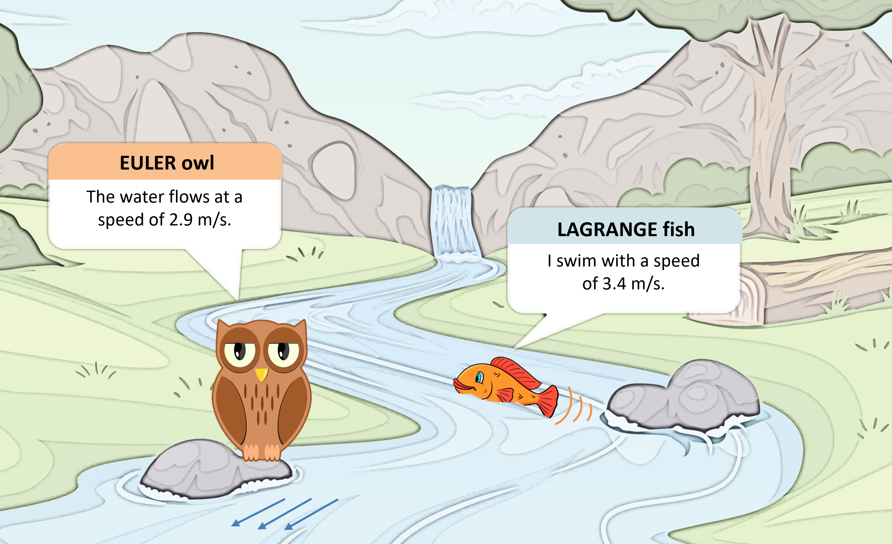
Figure 7.11: The description of movement processes depend on the perspective: Eulerian movement is the flow of a continuum at a certain location, whereas Lagrangian movement describes the trajectory of a moving entity.
7.4.1 Vector fields
Let’s take a stationary (Eulerian) view on each cell in a grid and determine the speed and direction of a force. The result is a grid of vectors. These vectors could represent wind, water flow or the magnetic field of the earth. A particle that is placed into this continuum of forces will be pushed like a leaf by the wind (Figure 7.12).
Go ahead and test, how vector field simulations operate.
Setupthe model to see a vector field. In our case it represents wind currents.- Press
place leavesand click on the canvas to place a leaf. Place as many leaves as you wish. - Hit
goto see how leaves are moved by the wind (Lagrangian motion). If the leaves don’t move, adjust the speed slider close to its maximum.
Figure 7.12: The vector field in this model represents the forces of winds that pick up a leaf and move it through the air. NetLogo Web
7.4.2 Advection
Advection processes describe how something is passively transported by a moving fluid (or air). The example of a leaf that is transported by the wind would be a typical advection process. It is the Lagrangian perspective of the model above. A typical application area for advection models is the process of erosion by wind or water.
The model in Figure 7.13 is part of the NetLogo model library. It simulates soil particles that are picked up and transported by water streams flowing down a hill. The result is fluvial soil erosion. The emerging erosion patterns will look familiar to you.
- Switch the
hill?parameter on andsetupthe model. - Hit
go - Without stopping the model, hit
setupagain andhide-water. Now you can see the pure advection (erosion) process without being hidden behind the flow process.
Figure 7.13: Fluvial soil erosion is an advection process. NetLogo Web