Lesson 9 Developing a model
This lesson zooms out from the operational perspective of how to program specific models and provides an overview on the entire modelling workflow. Starting from the problem to be solved, the design of the model, its implementation, testing, calibration, validation and finally the analysis of simulation outcomes. This workflow usually is not linear, but cyclic in nature: a first, basic model may be buggy and flawed, and often is also too simplistic to answer all questions. The modelling workflow thus is also referred to as the modelling cycle. This lesson provides the main idea, while the upcoming lessons will add more detail and practical tips on what needs to be done in each of the steps of the modelling cycle.
Upon completion of this lesson, you will be able to..
- approach the development of a model in a systematic way,
- overlook which methods need to be applied, and which software can be used, and
- efficiently plan and coordinate the tasks that are involved in a simulation modelling project.
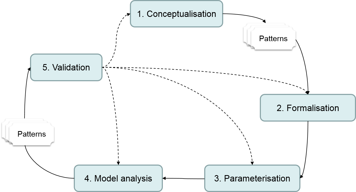
Figure 9.1: The five steps of the modelling cycle to develop a simulation model.
It has proven successful to take a rapid prototyping approach, i.e. to quickly produce a simple prototype by reusing existing building blocks, to parameterise it with plausible values and run a first simulation. After subsequent analysis and validation of the first results we will already have a good grasp on what the model does and what is still missing. Probably we need to re-conceptualise parts of the model, add code, refine parameters etc.: we are going to iterate through the ‘modelling cycle’ many times until the model is good enough for the purpose it is designed for.
9.1 Design of a conceptual model
The conceptual model is the most fundamental level to describe and discuss a model. Not surprisingly, also the most fundamental kinds of error and uncertainty are related to the conceptual model of the system. It specifies system components, their interrelationships, the temporal and spatial scale and the boundaries of the system, the input parameters, state variables, and expected outputs. Last but not least, this is the phase in which a modeller identifies the patterns that will be used for validation: which obsereved data is available against which simulated patterns can be tested?
The design of a conceptual model specifies in detail how a system is represented in a computer model to meet a specific purpose. The modeller explicitly declares and reasons about all these decisions and assumptions of the conceptual model. In the next lesson, I will provide a “cookbook” to assist a systematic approach to designing a new model.
9.2 Formalisation
Formalisation refers to the process of translating a conceptual model into a computer-readable ‘language’. Depending on the approach, a model can either be formalised with code (Figure 9.2), like in cellular automata and agent-based models, or by defining mathematical equations, like in system dynamics models.
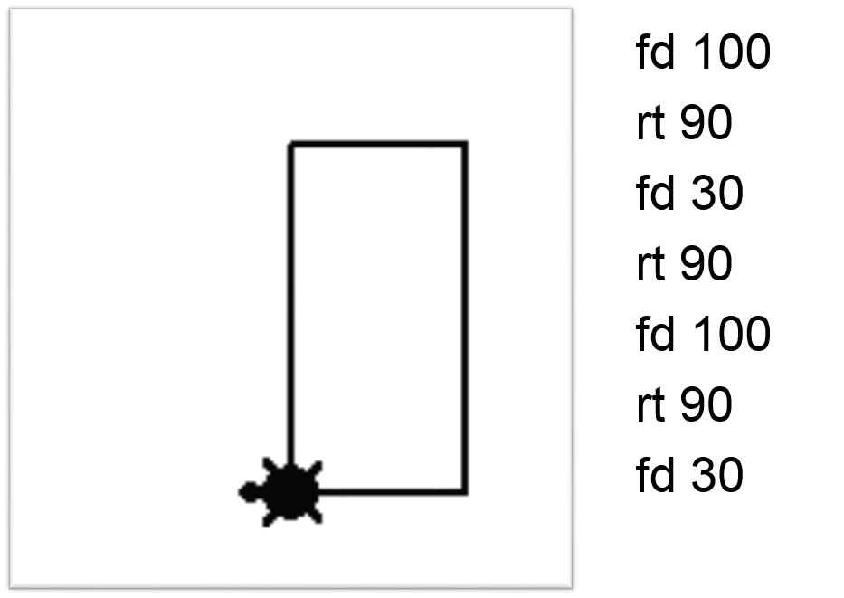
Figure 9.2: Formalisation transfers a conceptual model into a computer-readable format. Here, the turtle draws a rectangle with a few forward (fd) and right-turn (rt) commands.
The main intellectual contribution of a model lies in the conceptualisation of the system, not in writing code. Therefore, in most cases modellers are experts in their domains, but they do not have any formal training in programming. Modelling frameworks have been developed to support modellers in writing model code. These frameworks come with a GUI, provide built-in calibration algorithms and visualisation tools. Some frameworks even offer domain-specific programming languages that are relatively easy to learn, but at the same time provide a powerful functionality for the specific purpose of building simulation models. We have got to know two of the most prominent examples in the open source domain, which are NetLogo and GAMA.
NetLogo was developed in the spirit of the educational Logo programming language family according to the motto ‘low threshold and no ceiling’. Despite its old-ish look and feel, it is a powerful ABM modelling framework under active development with a couple of very nice features, like NetLogo Web. This makes it possible for me to share with you iFrames of self-coded model examples in this module. Thanks to its ease of use, it is probably the most widely spread framework in the research community. It offers a GIS extension that allows to read geographic data. Following the spirit of building on educational programming languages, the GIS functionality borrows from My World GIS, which was developed for the use in middle schools. Unfortunaltey, this limits the capabilities of NetLogo to seriously work with geospatial data.
The Repast Suite is another wide-spread open-source ABM modelling framework. The core software “Repast Symphony” is Java-based and thus more demanding in terms of required programming skills. For large-scale models, it is worth looking into Repast HPC that allows to design models that can be distributed over several cores for high performance computing. This is clearly for expert users, as the modeller needs to have a good understanding of load balancing in distributed computing systems. Models in Repast HPC are coded in C++. Repast4Py offers a python interface to Repast HPC. More relevant for GIS professionals: Around 2010 there has been an attempt to integrate Repast Symphony with ArcGIS by means of the AgentAnalyst plugin for ArcMap 10, but with new ArcGIS releases the plugin wasn’t further developed.
Finally, GAMA (GIS and Agent-based Modelling Architecture) has its focus on spatially explicit simulation and it provides the richest GIS functionality. By now, you know this framework well. In case you want to continue working with ABM modelling and GAMA, you will discover many more great functionalities, like user interaction, the integration of equation-based (system dynamics) models, benchmarking for computational optimisation, automated optimisation methods for calibration, or the support of some conceputal modelling approaches like the advanced driving skill, or the BDI (“belief-desire-intention”) framework.
AnyLogic is an example for a commercial agent-based modelling platform. It sticks out through its support for multi-method models, integrating agent-based, discrete event and system dynamics modelling. A focus application area for AnyLogic is logistics, including models of the transporation and storage of goods via rail, road or pipelines. There is a free student license that offeres basic functionality.
Modelling frameworks and model code-sharing platforms provide an increasing wealth of model libraries that serve as building blocks for more complex models. This takes away the hurdle of coding from scratch for each new model. However, model libraries are specific to the modelling framework, you are working with and thus are hardly transferable.
On a more general level, modellers often share prototypes and sample models on online platforms with open licences. These models have the advantage of being intensively tested and verified and thus are the basis of a collaborative effort of the modelling community to advance the field as a whole. The most establised cross-platform network and model sharing platform is CoMSES.
9.3 Parameterisation
Parameterising a model is like sitting in the front of a dashboard and turning the knobs before starting the show.
A parameter is an invariant input variable that represents a property of the modelled system.
In the parameterisation, all parameter are assigned an (initial) value. For example the parameter ‘tree growth per year’ may have the value of 20 cm per annual time step. Unlike variables, which change over time during simulation depending on the respective state of the system, parameters are either completely invariant or their variation is specified externally beforehand, e.g. to model an environment with constantly increasing temperature.
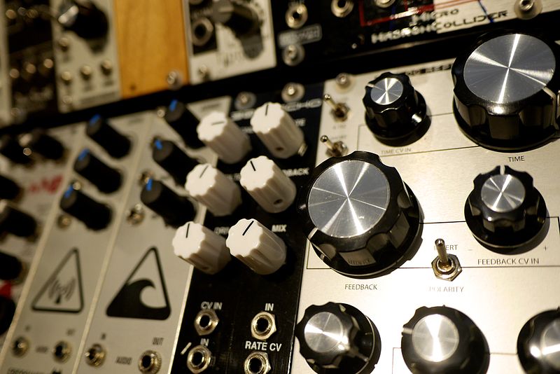
Figure 9.3: Parameterising a model is turning the knobs of the model’s dashboard.
9.4 Model analysis
The output of a simulation run usually consists of a large amount of numbers, that is: data. These data describe the state of the system over time and the emergence of patterns at system level. However, to retrieve this information from the simulation data, we need to analyse it. Or as Grimm and Railsback (2005) put it: we need to decode the data to extract the information, i.e. the expected patterns. Thus, the adequate portrayal of emergent patterns is the core task in this modelling step.
A state variable is a variable, which characterises the current state of a system or an entity in the system.
Printed over time, state variables visualise the dynamics of a system. A set of state variables describe a pattern. Taken together they can then be used to define the “state” of the system or model respectively.
A pattern is a spatio-temporal phenomenon “above random” that describes emergent properties of the system. Simulated patterns are often used for validation by comparing them with patterns that can be observed in the real system.
9.5 Validation
The validation is the last step of a modelling cycle: here, we check the validity of the model outcome. There are many strategies for model validation and we will dedicate an entire lesson to it. However, for the time being, we assume that we validate the quality of the model by comparison against reality. This is the most rigorous way of validation and can be seen as default strategy for applied models. The validation is thus based on the comparison of state variables and spatio-temporal patterns between modelled and real systems.

Figure 9.4: In validation, we compare the model outcome with reality.
There are two possible results of the validation step:
If the model does not yet produce valid results, we will try to address the modelling step that contributes most to the deviation of the model from the real system. This is part of an overall validation strategy and will be discussed in more detail in a later lesson.
If we conclude from the comparison between model and the real-world system that the model is valid with respect to its purpose, we can stop the modelling cycle and proceed to use the model for our research.