Lesson 14 Scenario-based research
In this lesson we draw everything together and go through the process of problem solving (i.e. conducting research) with simulation models. In the research workflow, the time consuming and demanding phase of model development is only the first step. A valid model does not provide us with any insights and its mere existence does not solve our research problem. In that sense, a model is nothing than a tool. Only the second step ‘scenario analysis’ produces the results we need to answer the research question. In fact, the scenario should already be embedded explicitly in the research question.
I refer to Shell (2008, p8) for a simple and elegant definition of a scenario:
A scenario is a story that describes a possible future.
A scenario can contain verbal descriptions of (changing) contexts, driving forces or events that lead to a future state. Again, it is on the modeller to pick relevant and interesting scenarios. Usually two or three alternative scenarios are enough to gain a lot of insights into how a system works.
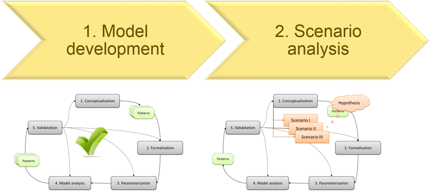
Figure 14.1: The workflow of conducting research with models.
14.1 Model development
14.1.1 Define research question
As the example to discuss the workflow of scenario-based research, we pose the question, whether soil erosion patterns on a slope depend on the temporal distribution of rainfall.
Our hypothesis is as follows: A few heavy rain events result in less, but deeper erosion patterns compared to constant drizzle rain that sums up to the same amount of rainfall.
14.1.2 Draft the conceptual model
As part of the conceptual model a first graphical representation of the two scenarios is provided (see Figure 14.1). If possible, it is always a good idea to support a verbal description of the model’s purpose with a graphical representation: it is the ‘graphical abstract’ of your work, which is intuitively understandable and thus very effective in communicating the key point of your research.
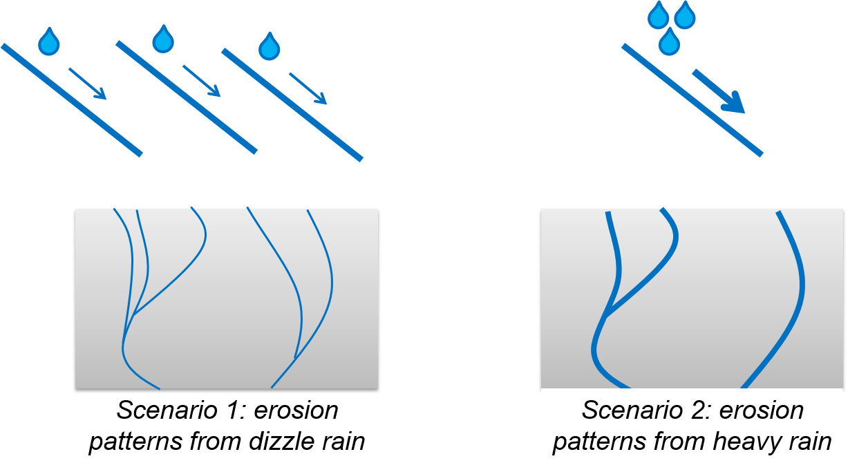
Figure 14.2: The research hypothesis determines the scenarios: a few heavy rain events result in less, but deeper erosion patterns (right) compared to constant drizzle rain (left) that sums up to the same amount of rainfall.
14.1.3 Specify the expected patterns
To specify, how to quantitatively measure the expected erosion patterns in the model outcomes as well as in the real-world, we identify a set of state variables. Let’s define the following five state variables to evaluate our model against reality:
- Number of eroded cells (=eroded area)
- Mean erosion depth
- Max. erosion depth
- Min. erosion depth
- Erosion volume (=amount of erosion)
As we have defined the state variables, we can check, whether adequate validation data are available. Lack of adequate data for model validation is a common risk for the success of a simulation modelling project. If we fail to get hold of adequate data, it is the right time to either adapt the model to match the validation data or to organise the collection of data that is needed.
14.1.4 Develop the model
We skip the rest of the model development phase, in which we iterate through the modelling cycle until the model is deemed to be valid for the purpose: this phase has been covered extensively in the previous lessons. Instead, we assume a successfully validated model and proceed directly to the second phase, the scenario testing.
14.2 Scenario testing
When we implement a scenario we need to specify its “story” with the help of parameters. In the case of “drizzle rain (Scenario 1 “drizzle rain”) vs. few heavy rain showers (Scenario 2 “heavy rain”) that sum up to the same amount of water” we may decide to model a constant amount of rain each day in a year vs three heavy rain showers on day 1, 50 and 100 of the year. The rainwater is distributed as random drops over an artificial slope. The ‘lab’ is set and the experiment is ready to run: let’s hit the “go” button!
14.2.1 Monte Carlo simulations of scenarios
We run each scenario once and compare the outcomes for two state variables, ‘number of eroded cells’ and ‘mean erosion depth’. The outcomes seem to support our hypothesis that heavy rainfalls indeed result in less, but deeper erosion patterns. However, as we have random distribution of the raindrops over the study area and some stochasticity in the run off, we will need to run a Monte Carlo simulation to get statistically valid results. Therefore, we set up a model experiment and repeat the simulations for each scenario one thousand times. An automatic routine saves the five state variables for each simulation run into a table.
Depending on our model and the number of iterations the simulation runs can take a while – time enough to go for a coffee, or sometimes even to take an extended walk in the woods. I can remember the door signs at the biology department of my graduate university “Experiment in progress – do not enter!” And sometimes, a swear of a frustrated Master student, who forgot a detail in the experimental setting and had to redo the entire experiment. Also in this respect a computer simulation is not very different from a lab experiment. So double check before you hit the start button!
Anyway, when we come back and everything went well, the outcomes of the scenarios hopefully wait for us. There we go: this is the outcome of our Monte Carlo simulation: two tables (one for each scenario) with five columns (one for each state variable) and 1000 rows (one for each simulation). It is like the raw data we get from a lab experiment. Let’s load the data and view the first 6 rows of one or the tables in R.
drizzle <- read.csv("documents/Erosion_scenario_drizzle.csv")
heavy <- read.csv("documents/Erosion_scenario_heavy.csv")
head(heavy)
## amount.of.erosion amount.of.eroded.patches min.erosion max.erosion
## 1 -221.703 21251 0 -0.147
## 2 -216.987 21655 0 -0.146
## 3 -217.724 20963 0 -0.146
## 4 -215.023 21562 0 -0.119
## 5 -217.261 21326 0 -0.197
## 6 -217.275 20996 0 -0.161
## mean.erosion standard.deviation.of.erosion
## 1 -0.002463367 0.010663198
## 2 -0.002410967 0.009851151
## 3 -0.002419156 0.010242233
## 4 -0.002389144 0.009718875
## 5 -0.002414011 0.010522370
## 6 -0.002414167 0.01072403514.2.2 Scenario analysis
We need to analyse the simulation data statistically to extract any useful information. When we plot the outcome of one of the five a state variables, we will see how the values of this variable are distributed. Already visually it becomes obvious that the state variable “number of eroded cells” is different between the scenarios. The drizzle rain scenario results in less eroded cells.
plot(density(drizzle$amount.of.eroded.patches), col = "blue",  xlim = c(18500,22500), main = "Amount of eroded area", xlab="eroded area in m2")
lines(density(heavy$amount.of.eroded.patches), col = "red")
legend("topright", c("Scenario: drizzle rain","Scenario: heavy rain"), lty = c(1,1), col = c("blue","red"))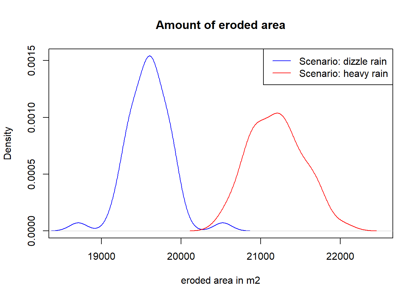
By means of a t-test we can compare the value distributions of the alternative scenarios statistically. T-tests are standard statistical methods that can be used to determine if the means of two data sets are significantly different from each other. If we are lucky and the data are normally distributed and of the same shape, the student’s t-test can be used. For normally distributed data of different shapes, the Welch t-test is more adequate. Non-normal distributions unfortunately are more difficult and we will not further discuss these cases here. However, our distributions are close enough to a normal distribution that we can use an Welch t-test (=a two-sample unpooled t-test for unequal variances, where ‘unpooled’ means that the two samples have unequal variances). In the statistical software package R this is the default for t-tests as this is the most common distribution. The command in R is quite simple, the results can be viewed below:
##
##  Welch Two Sample t-test
##
## data:  drizzle$amount.of.eroded.patches and heavy$amount.of.eroded.patches
## t = -25.772, df = 92.164, p-value < 2.2e-16
## alternative hypothesis: true difference in means is not equal to 0
## 95 percent confidence interval:
##  -1726.221 -1479.207
## sample estimates:
## mean of x mean of y
##  19592.59  21195.31
The results can be interpreted as follows: The hypothesis of the t-test is that there is no difference between means of the samples. The p-value states, whether this hypothesis is true. For p < 0.05 (the 5% confidence interval) the means are likely to be different. In our case the p value is much smaller than 0.5, in fact it is almost zero. So we can conclude, that there is a highly significant difference between the scenarios. The last two lines provide the mean eroded area of the two samples: 19592.59 m2 for the drizzle rain and 21195.31 m2 for the heavy rain scenario.
Let’s do the same analysis for the erosion depth:
##
##  Welch Two Sample t-test
##
## data:  drizzle$mean.erosion and heavy$mean.erosion
## t = 7.2172, df = 88.929, p-value = 1.704e-10
## alternative hypothesis: true difference in means is not equal to 0
## 95 percent confidence interval:
##  4.199718e-05 7.390715e-05
## sample estimates:
##    mean of x    mean of y
## -0.002347567 -0.002405519
Again, the results show that the erosion depth in the two scenarios is significantly different, where the heavy-rain scenario has marginally deeper erosion: 2.4 compared to 2.3mm depth after one year.
So, let’s revisit the hypothesis: “Heavy rain results in less, but deeper erosion.”. This hypothesis needs to be rejected and reformulated: “Heavy rain results more and marginally deeper erosion”.
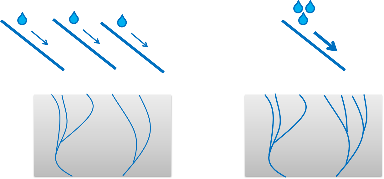
Figure 14.3: The ‘’new hypothesis’’ can be formulated as: ‘Heavy rain results in more and marginally deeper erosion’
14.2.3 Insights gained
So, what do we conclude from these results? The statistical basis is sound, so we are confident that the results give a correct insight into the modelled processes. Further, we have thoroughly validated the model and we think it adequately represents the real world. Therefore, we are confident that the model results provide new insights into run-off processes. However, it still is a model and our new hypothesis needs to be tested in physical experiments and / or real world contexts.
To wrap up, working with agent-based models most often implies working with stochastic models that need to be analysed statistically. Scenario analysis provides you with the expected results and insights regarding your geospatial process of interest: this can work into the future as well as into the past (Figure 14.4).
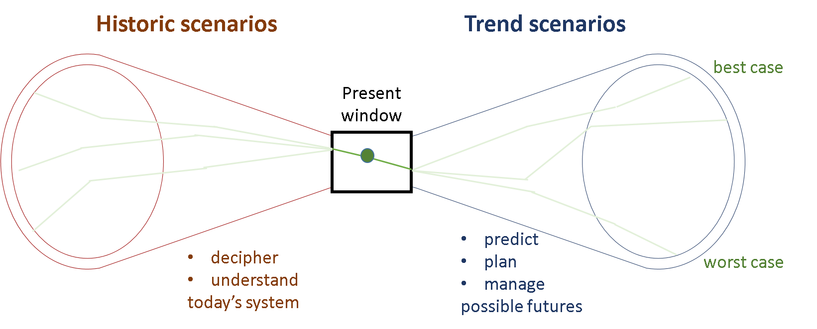
Figure 14.4: Step by step, scenario analysis can contribute to a better understanding of the processes that shape our complex world.