Lesson 2 System dynamics
System dynamics is a mathematical modelling technique that is rooted in the General Systems Theory. System dynamics was developed to frame, understand, and discuss complex issues and problems from the perspective of systems theory. It was the first simulation modelling approach that was developed and it greatly influences modelling communities across all domains until today. This lesson introduces to system dynamics modelling by relating to the three conceptual components of a system’s model: purpose, elements and relations. The lesson then looks into typical system behaviour and implications for dealing with systems.
Upon completion of this lesson, you will be able to..
- conceptualise a system with its stocks, flows, and feedback loops in a causal loop diagram.
- identify growth, decay, steady states and oscillation the underlying processes of complex system behaviour, and
- finally, “read” the mechanisms behind more complex system archetypes and be aware of the implications for living in and interacting with systems.
2.1 System dynamics modelling
2.1.1 Purpose
The purpose for which system dynamics was developed is to increase understanding of the dynamic behaviour of systems.
System dynamics is a mathematical simulation modelling approach with the core assumption that complex, non-linear behaviour of systems can be explained with a set of relatively simple processes that govern flows of energy and matter between interrelated, homogeneous sub-parts (stocks) of the system (Figure 2.1).
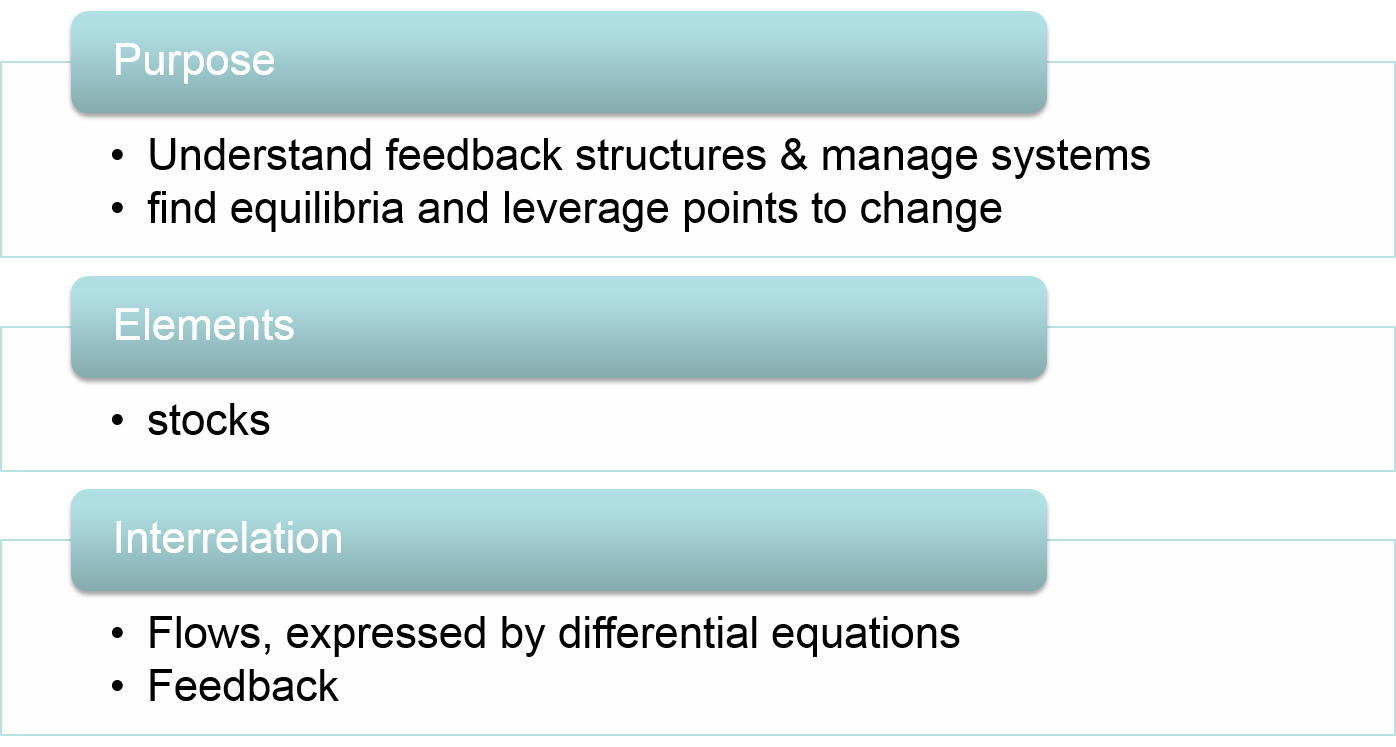
Figure 2.1: With respect to the three components of a system (elements, interrelations, purpose), a system dynamics model consists of stocks (=elements) and flows (=interrelations).
System Dynamics was developed by a group of researchers around Jay Forrester and Donella Meadows at the Massachusetts Institute of Technology (MIT) in the 1950s (Figure 2.2). In the absence of computers at that time, the scientists had to work with tedious hand simulations. Gladly, they took advantage of computers in the early days of this technical revolution.
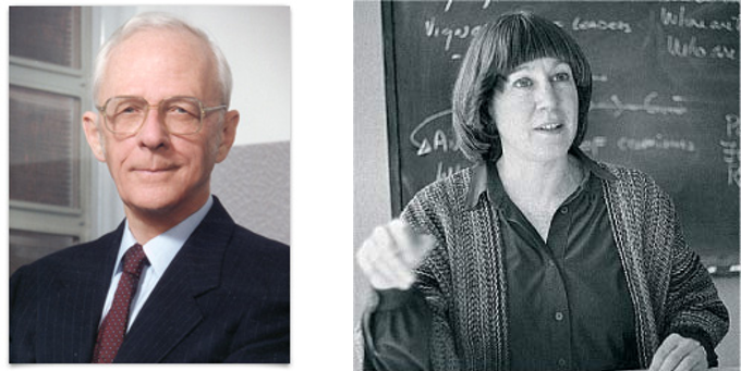
Figure 2.2: Jay Forrester (1918 - 2016) and Donella Meadows (1941 - 2001) developed the system dynamics modelling approach.
2.1.2 Elements: stocks
Stocks are the core building blocks of system dynamics models. A stock is a homogeneous part of a system that holds a measurable amount of something in which we are interested – just like a container or system’s storage room. Examples for stocks are water in a lake, animals in a population, or money in a market. Stocks are easily recognised in a system and thus are a good starting point to conceptualise a system dynamics model.
Stocks by design assume average values across space. Although there have been attempts to tesselate space to some degree for designing spatial system dynamics models, the focus is given to dynamic patterns in the temporal domain.
However, the basic concepts of system dynamics are extremely helpful to understand models of complex systems. In this lesson, we will therefore explore some typical system dynamics models before we then move on to spatially explicit modelling approaches in the remainder of this module.
2.1.3 Relations: flows
Flows are ordinary differential equations that model, how stocks are linked together. Depending on the flow process, the stock grows or declines, oscillates or develops towards an equilibrium. Typical examples for flows are births and deaths, purchases and sales, growth and decay.
Let’s have a quick look at the maths behind flows: in ordinary differential equations, we describe how a variable evolves over time. These differential equations cannot be solved analytically. This means, there is no way to use mathematical methods to come up with an exact solution. Instead, we need to dissect time into small slices and calculate the linear difference between these time steps. So we turn a non-linear differential equation into small steps of linear difference equations. This stepwise approximation is referred to as the Euler method (Figure 2.3).
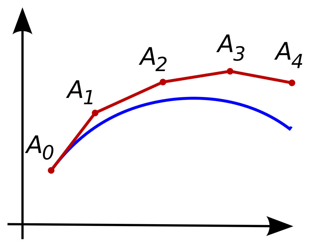
Figure 2.3: Numerical simulation is the iterative approximation of differential equations with the Euler method. Image source: Oleg Alexandrov, Wikipedia
The Euler method takes an initial value from where it starts to solve the first difference equation. Taking the result it then iteratively solves the next equation, and the next, and the next, etc. This mathematical approach is called numerical simulation. The smaller the time steps, the more accurate is the result. System Dynamics software thus is a tool for numerical simulation of ordinary differential equations.
2.1.4 Stock and Flow diagram
A major asset of System Dynamics modelling software besides solving the ordinary differential flow equations with numerical simulation is the use of declarative modelling environments. These environments enable a modeller to use graphical representations of the system rather than writing equations and programming code. This convenient way of representing a system in a computer-readable form is termed ‘Stock and Flow diagram’. Figure 2.4 shows the notation rules to design a stock and flow diagram.
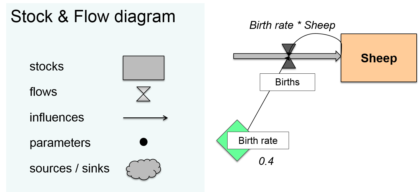
Figure 2.4: Notation rules of a Stock and Flow diagram.
- Stocks
- Flows
- Influences show causal relations: which parameters / stocks influence a flow.
- Parameters quantify the ‘valves’ of a flow. Flows can increase or decrease – depending on the rate of change. By ‘turning the valves’ we manipulate flows.
- Sources and sinks represent the boundaries to the environment around a system. As we work in open systems, there is always an ‘outside environment’ that functions as source and/or sink.
2.1.5 Feedbacks
Feedback loops the key mechanisms to govern system behaviour. There are two types of feedback, reinforcing feedback accelerates and self-regulating feedback balances a system.
In the first case, we have a system with one feedback loop, which is a self-reinforcing (positive) feedback (Figure 2.5). It has positive causal links of the form ‘the more – the more’: the more sheep, the more lambs are born. The more lambs, the larger the population. The result represents the deregulated behaviour of a system: the population grows exponentially. An example for this dynamic behaviour are bacteria that are cultivated on an agar plate. Under good environmental conditions, bacteria are immortal. As long as these bacteria are not limited by the availability of nutrients, the growth dynamics is exponential. However, a self-reinforcing feedback can equally well have negative causal links of the form ‘the less – the less’, resulting in an exponential decay.
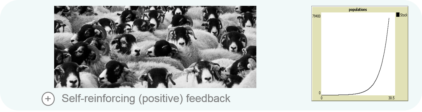
Figure 2.5: Self re-inforcing (positive) feedback is the ‘engine’ that causes a system to grow
In the second case, we also have only one feedback loop. This time it is a self-regulating (negative) feedback (Figure 2.6). The result is a stabilisation of the population at a certain level: the population decreases proportional to its current value. The dynamics takes the form of an exponential decay. In this case, without any inflow, the sheep population approaches zero.
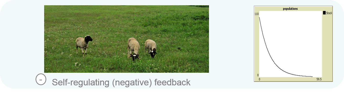
Figure 2.6: Self-regulating (negative) feedback balances a system towards equilibrium
2.1.6 Causal Loop diagram
For identifying feedback loops when designing the model of a more complex system, modellers often make use of sketching the system of interest in a “Causal Loop Diagram” as a prior step, before operationalising the model into a Stock and Flow diagram.
To construct a Causal Loop diagram, the modeller sketches the “story” of the system: he writes down the “nouns”, that is the name of the stocks and in between the flows, which are the “verbs” and places an arrow to indicate the direction. Then, parameters are added, again with an arrow to indicate the variable which the parameter influences.
By the example of the Causal Loop Diagram in Figure 2.7 the “sheep” -> “give birth to” -> “sheep”, where the “birth rate” influences the “birth” flow. The connections between the variables can be positive in the form of a ‘the more – the more’ or ‘the less – the less’ relationship, e.g. the more births, the more sheep. Negative relations direct into opposite directions in the form of ‘the more – the less’ or ‘the less – the more’, e.g. the more deaths, the less sheep are in the population. The according + or - sign is written next to the arrow tip.
Once all influence arrows build a circle in the same direction, there is a feedback loop. To determine, whether it is a self-regulating, or a reinforcing feedback, just count the minus signs in the loop: if there is an odd number of minus signs (one, three, five, etc.) it is a self-regulating loop, otherwise it is a reinforcing loop.
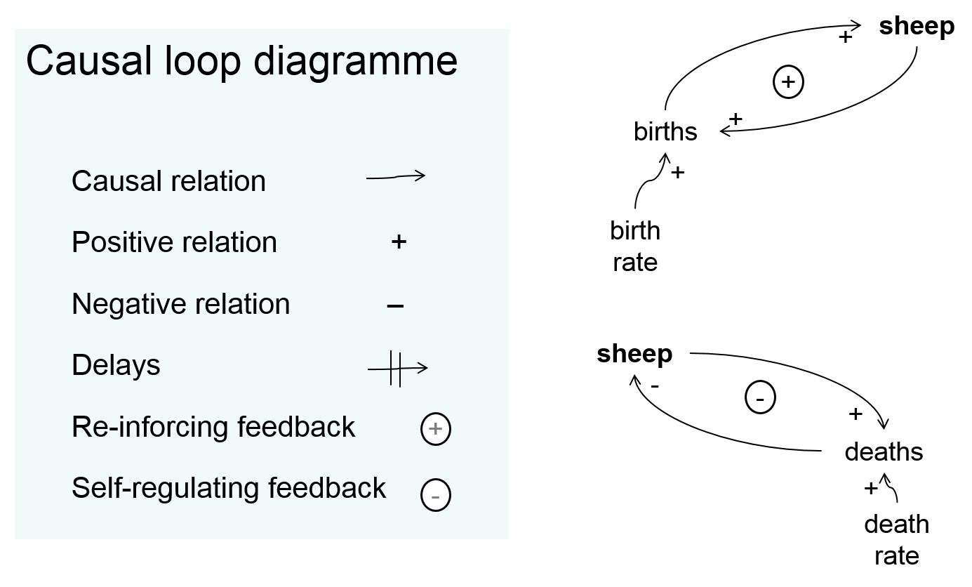
Figure 2.7: Notation of Causal Loop diagrams
2.2 System behaviour
System dynamics model are very well suited to study the elementary ways in which a system can behave: linear growth, exponential growth, logistic growth, equilibrium (or: steady states) and oscillations (Figure 2.8). These processes govern systems and you will encounter them in all systems, regardless of the domain or the type of application.
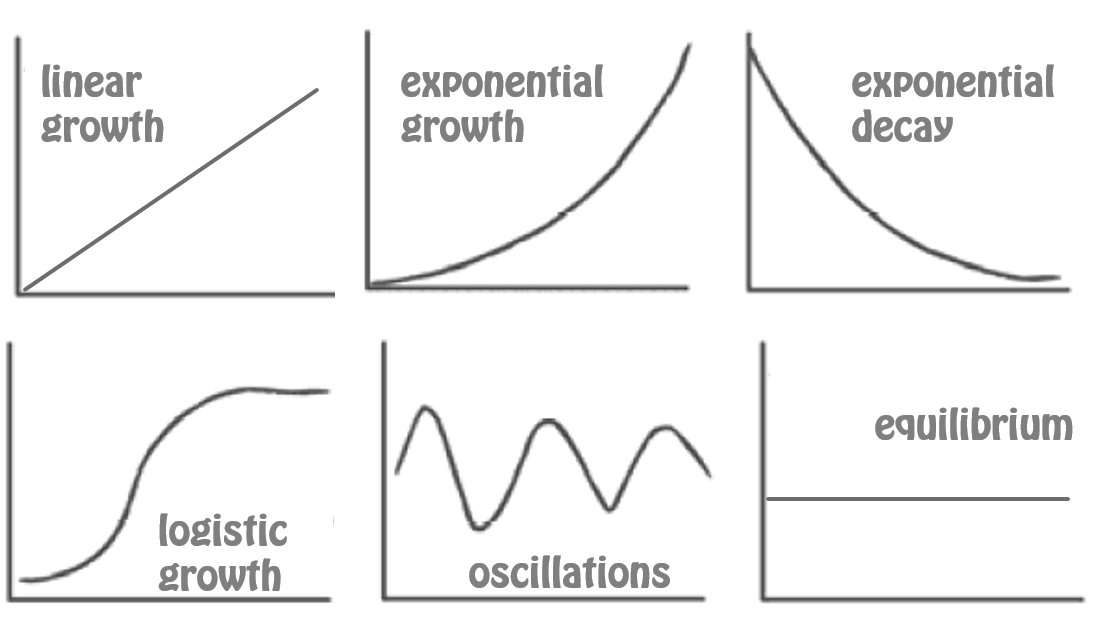
Figure 2.8: The six basic processes that result from flows between stocks.
More complex system behaviour is always a combination of these simple process types. When we take multiple ‘simple’ concurrent flows to connected multiple stocks in a system, the resulting system behaviour will quickly grow to a complex, non-linear behaviour. However, these process types are not limited to system dynamics modelling. Later, when we turn to Geosimulation of spatial systems, you will observe, how growth, oscillations and steady states emerge from the local interaction between individuals.
2.2.1 Growth and decay
Linear growth or linear decrease results from constant inflow or outflow that is not related to the amount of the stock. An example would be migration. Mathematically, linear growth is described as follows:
Pt+1 = Pt + dt
The amount of P in the next time step will be the current amount of P plus the difference per time step.
In GAMA, you would simply write:
// P increases by x each time step
P <- P + x;
Exponential growth or exponential decay results from inflows or outflows that depend on the amount of the stock. We have encountered these processes in relation to feedback: self-reinforcing feedback always leads to exponential growth, whereas balancing feedback results in exponential decay. Mathematically, exponential growth is described with a stepwise approximation of diffential equations with difference equations.
Pt+1 = Pt + r * Pt
The amount of P in the next time step will be the current amount of P multiplied by the rate at which P grows each time step. Growth rates above zero result in exponential growth and rates below zero result in exponential decay,
In GAMA, you would write:
// P increases with the growth rate r
P <- P + r * P;
Logistic growth or logistic decay results from inflows or outflows that depend on the amount of the stock AND the carrying capacity of a system. Logistic growth starts off just like exponential growth, but the closer the state of the system approaches its carrying capacity, the more is the growth slowed down until it reaches a steady state. Mathematically, logistic growth is described with a stepwise approximation of differential equations with difference equations.
Pt+1 = Pt + r * Pt * (1 - Pt / K)
The amount of P in the next time step will be the current amount of P multiplied by the rate at which P grows each time step (=exponential growth) multiplied by the following clause: 1 minus the quotient of the current amount of P and the carrying capacity K. The latter clause approximates zero the closer P gets to the carrying capacity, and consequently Pt+1 cannot grow beyond K.
In GAMA, you write:
// P increases with the growth rate r
P <- P + r * P * (1 - P/K);
2.2.2 Equilibrium
Each living system has its own steady state in which internal conditions are stable and remain constant within amazingly narrow boundaries. For example, the temperature of a human body usually is just a little lower than 37°C. If this temperature rises by just a few tenths of a degree, we feel uncomfortable. If our body temperature is three to four degrees off, we are seriously ill. This tight temperature regulation works, no matter whether the air temperature around us is at +40°C or at -10°C. The same stable balance holds true for the levels of glucose in our blood, the calcium levels, and the blood’s pH. This very stable steady state in the physiology and metabolism of living organisms is called Homeostasis (from Greek for ‘similar state’). Only, if we expose ourselves too long in extreme conditions, our body cannot keep the balance and the system eventually collapses.
Figure 2.9 shows different types of equilibria. Homeostasis is an example for a stable equilibrium that is caused by balancing feedback loops, which push a system to progress towards its equilibrium and to get back to this equilibrium after disturbance (stable equilibrium). Whereas, dynamic equilibria are a special case, that are rare in real systems: inflows and outflows need to be at the exact same rate. If there is just a small imbalance, the system will develop in the one or the other direction.
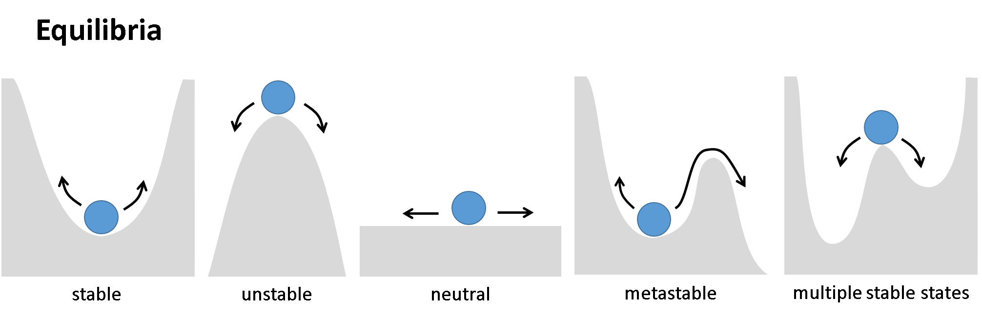
Figure 2.9: Equilibrium concepts
General Systems Theory starts from the premise that this phenomenon of stable steady states is also inherent to living systems at higher organisational levels, i.e. populations and ecosystems. As long as nature is in balance, an ecosystem will tightly control the flows of material and energy and its stocks will be balanced at a certain level. The steady state of a population that can be sustained by the resources in a certain ecosystem is called the carrying capacity of this ecosystem.
If a disturbance event results in an ‘unsustainable’ number of animals or humans in that population, the ecosystem has the capacity of regulating itself and recover its balance (resilience). However, if the disturbance exceeds a certain limit, the ecosystem collapses. The balance of nature paradigm has been under debate (e.g. Wu and Loucks 1995), as things are always evolving and developing - not just since we witness climate change. Steady states are thus helpful to conceptualise a system, but in practice systems are rarely in steady states. Today, the concept is complemented with more bottom-up process oriented views related to complexity theory.
2.2.3 Oscillations
Last but not least, we look into oscillations. Oscillations in a system can have two causes:
Oscillations by delay. Such oscillations can be seen, even if there is just one stock involved. An example are dangerous glucose levels after delayed insulin injections in diabetes patients (Figure 2.10). Similar oscillations can be found for delayed feedback reactions in all systems that are governed by balancing feedback loops, e.g. delayed orders and deliveries after an increased sales rate of a particular product; delayed reaction to changing temperatures in furnace systems; delayed reactions of a hunter to control a resource-limited deer population.
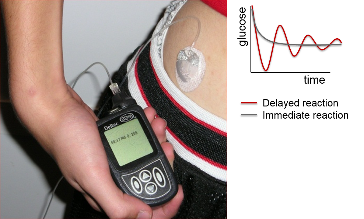
Figure 2.10: Insulin oscillations in a diabetes patient, who injects insulin late.
Oscillations by two interacting stocks. An example are disease outbreaks, in systems of interacting viruses and humans - we have seen this a lot during the Corona pandemic. Probably the most famous example of a two-stock, oscillating system is the predator-prey model. It was first formulated independently by two scientists in the mid 1920s. First, Alfred Lotka, who’s work was very influential to the academic world, although he followed a non-academic career and worked as a statistician at the Metropolitan Life Insurance Company most of his life. Second, Vito Volterra an Italian mathematician, who wondered about the oscillations of the availability of certain fish species in the Roman fish markets. The equations are today known as the Lotka-Volterra model. It is one of the most cited model in Ecology and it has inspired generation of researchers. The theoretical relation between a predator and a prey population has been proved empirically for many systems since, for example the abundance of snowshoe hare (Lepus americanus) and lynx (Lynx canadensis) pelts traded with Hudson Bay Company (Figure 2.11).
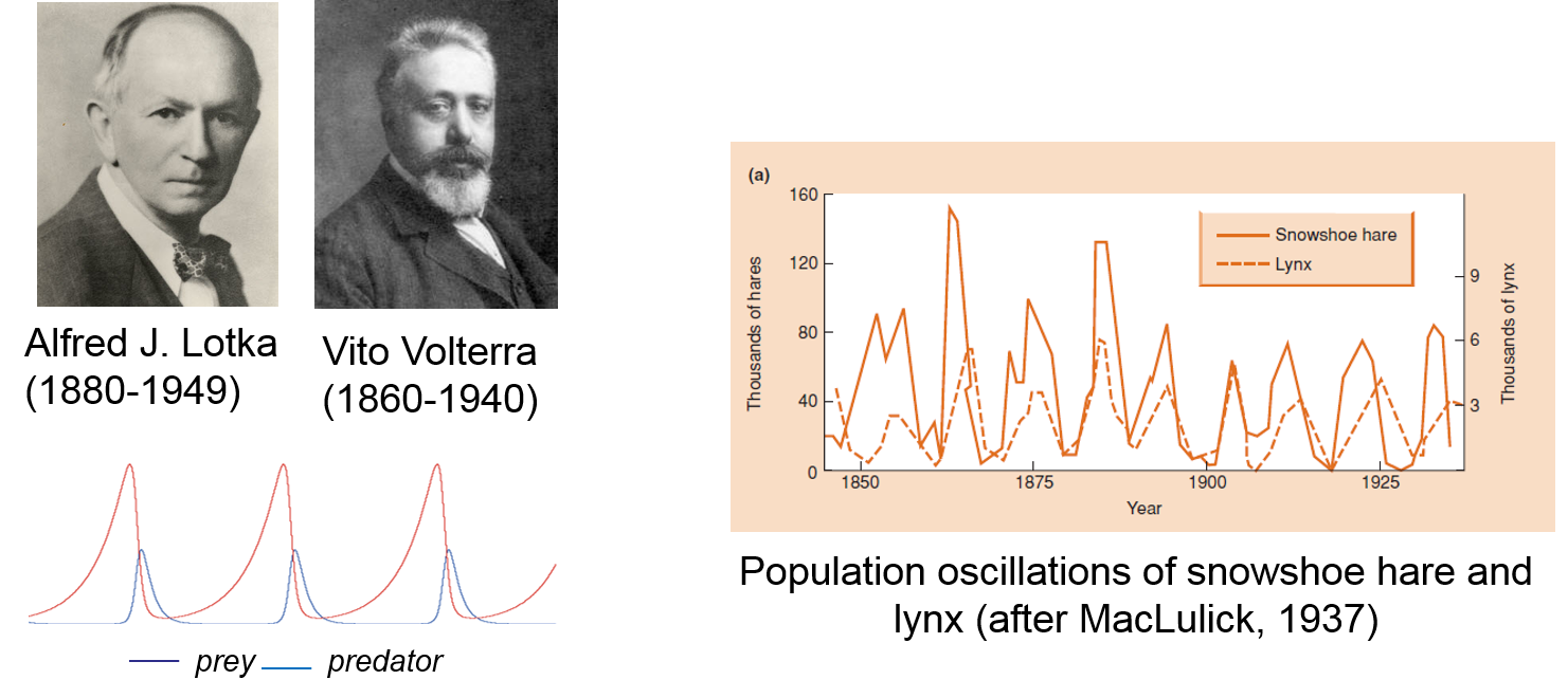
Figure 2.11: The famous Lotka-Volterra model represents the oscillations that emerge from the coupled populations of predators and their prey in an ecosystem.
2.3 Implications of Systems Thinking
Following from system theory, a system is governed by its internal state, its stocks and flows, rather than by outside forces. Take a moment to think about the implications of viewing the world through the “system lens”:
- Bark beetle invasions do not damage forests. It is the single-species, same-aged forest structure optimised for the timber industry that facilitates the damage.
- Political leaders do not cause economic booms or recessions. Ups and downs are inherent in the structure of the market economy.
- The flu virus does not attack you. The overworked guy in Figure 2.12 may just set up the conditions for a virus to flourish within his body.

Figure 2.12: Systems thinking, demonstrated by the example of the flu. An overworked body is highly susceptible to getting sick, while it is often easier to fight the virus as the culprit that causes all the trouble and thus need to be eliminated.
Psychologically, it is often easier to assume that a problem is ‘out there’ rather than ‘in here’. We would like to have a ‘control knob’ to solve a problem and blame somebody or something for causing a problem: flu viruses, bark beetles or politicians. Systems theory teaches us that things are not that simple and that we have to think differently, if we want to understand – and manage – systems.
Let’s have a look into some archetypical examples for the behaviour of (simple) systems from the perspective of Systems Theory. Well known system archetypes are Limits to Growth, Tragedy of the Commons, Eroding Goals, Shifting the Burden, Success to the Successful, or Escalation. You will find an Insight Maker model showcasing each of these archetypes. Here, we will look at three of them: Limits to Growth, the Bullwhip Effect and the Tragedy of the Commons. There is a story to each model explaining the functionalities of the models. So just go ahead and click on the ‘Start Story’ on the bottom left.
Insight Maker online modelling tool
Insight Maker is free online platform for creating models and simulations. It allows users to create system models and share them online with others. You just have to create a profile and can start modelling. Insight Maker works mainly with drag and drop objects which you can alter and adapt. So it is easy to use and does not require you to know how to code.2.3.1 Limits to Growth
Let’s start with the “limits to growth” system archetype (Figure 2.13). On the left side, there is a reinforcing feedback process that causes exponential growth. However, on the right side the system is balanced out by a negative feedback loop. The halt of the growth is imposed by limited resources: a commonly encountered system that keeps a stock within its limits.
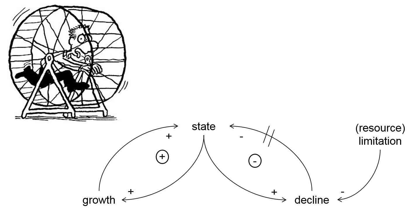
Figure 2.13: Limits to Growth model
Sometimes we want to go beyond these ‘natural’ limits. We want to run faster and faster to win that competition. We want to produce more and more corn on the same piece of land. We expect better and better performance of an employee. However, as we fail to properly acknowledged the limits of a system, we have to push it harder and harder. The former methods are continuously applied, but more and more aggressively. Most of the effort vanishes through the self-regulating feedback loop on the right.
Explore the interactive Limits to Growth model in Insightmakeer (Figure 2.14). You can think of agricultural food production as an example for this model.
Can the limitation be overcome? Think about what may happen, if you do so? Run a simulation with the default values and then try out to push the limits by dragging the limiting-factor slider from 20 to 50. Simulate again and compare the results.
Figure 2.14: Limits to Growth model, provided by Gene Bellinger
See solution!
A (short-term) solution in overcoming this limitation can lie in the weakening or elimination of the causes of limitation, for example through fertilisation of agricultural fields. In this model, we can successfully push the limits and gain higher results.
In real systems, the limits cannot be pushed endlessly: the system will face new limitations. A danger lies in a delayed feedback from the declined system to its state, which leads to oscillations that can go beyond system boundaries and eventually cause the system to collapse. However, these considerations have not been built into the model.
2.3.2 Bullwhip Effect
Sometimes, production companies are faced with insane oscillations of the demand, which can be a real problem. This is called the “Bullwhip effect”. So, what happens?
Let’s say a grocer sells 10 bottles of milk on Monday. On Monday evening he places an order to buy 10 bottles of milk that are missing in his shelves. On Tuesday he sells another 5 bottles. On Tuesday evening he gets a bit nervous and orders 7 bottles instead of 5 – just to be on the save side. On Wednesday he sells 15 bottles and he gets really stressed: almost no bottles are left in his shelves, so he sits down and orders 25 bottles. On Thursday the delivery man comes and brings 42 bottles of milk; 12 bottles too many than the storage room can hold and the shelves are jammed. The grocer decides to wait with any new orders until he has sold so many bottles that there is enough storage room again.
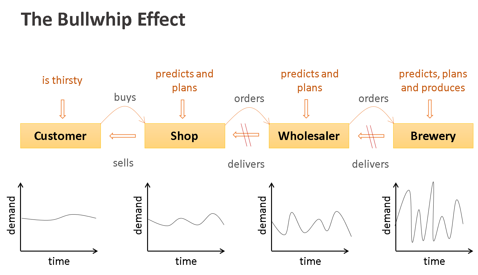
Figure 2.15: The Bullwhip Effect in production demands is an implication of delayed feedback in a supply chain.
When you plot the grocer’s stock over time, you will see a heavy oscillation. This oscillation is due to the delays in placing the order and the delivery of the product. Imagine, there were a milk pipeline that automatically refilled the milk, right after a customer had taken it out of the shelf: there would not be any oscillation in such system. Oscillations due to delayed deliveries are actually is quite common and pose a challenge to any stockholder. The oscillation gets ever more exaggerated the more levels of sale – and resale are involved. This effect is called the ‘Bullwhip Effect’. In studies conducted with a simple four-step supply chain, small variations in initial demand lead to order amplitudes of 900 percent (!) only four steps down the supply chain (http://www.shmula.com/the-bullwhip-effect/310/).
Play the beer game!
In the exercise, you play the beer game against the computer: try to have enough beer in stock and at the same time lower your storage costs.
2.3.3 Tragedy of the commons
The last system that we will discuss in this lesson is known as the „Tragedy of the commons“. The ‚commons‘ are community-shared goods, for example a piece of land that belongs to the aggregate members of a community instead of an individual land owner. Let‘s consider two farmers, who let their cattle graze on the commons. The more cattle farmer A sends to the commons, the more he will gain. The same is true for farmer B. The total amount of cattle of all farmers in the community is the ‚total activity‘ on the commons. If there was no resource limitation, everything would be fine. However, due to limited resources there is a negative relation between ‚total activity‘ and ‚gain per individual activity‘. The more cattle are on the commons, the less grass is there for each single animal and the gain per animal diminishes. Unfortunately, until the agricultural land collapses completely the individual farmer still gains more the more cattle he has on the commons.
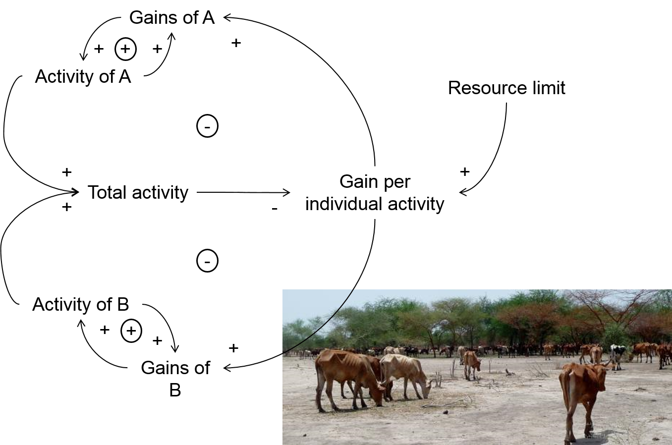
Figure 2.16: Tragedy of the commons
Many communities therefore put regulations into place, when and how the commons can be used by a member of the community in order to avoid a system collapse. A prominent example is the strict set of rules on the use of irrigation water in dry areas.
Figure 2.17: Tragedy of the commons model, provided by Gene Bellinger
2.4 WORLD 3 model
To finish off this lesson, I want to present the probably most famous system dynamics model, the WORLD 3 model. In the early 1970s the global think tank ‘Club of Rome’ asked Jay Forrester to develop a model of the world’s dynamics – the starting point of the Forrester-Meadows ‘WORLD’ models and the ground-breaking publication ‘The Limits of Growth’ (Meadows et al. 1972). The purpose of the model was nothing less than the ‘predicament of mankind’ and to learn about carrying capacities of our planet.
Limits to Growth
Donella ‘Dana’ Meadows is the lead author of the influential book ‘Limits to Growth’ (Meadows et al. 1972). This best-selling book in the 1070ies reported the insights gained from the WORLD 3 model that aimed at showcasing scenarios of the world’s development. Dana Meadows co-developed the model with Jay Forrester and other researchers at the MIT System Dynamics Group on behalf of the Club of Rome. Particularly interesting is a comparison with observed data in a 40year update by Turner (2014) and an update of the model’s predictions based on the state of 2023” with using this link: https://onlinelibrary.wiley.com/doi/full/10.1111/jiec.13442.
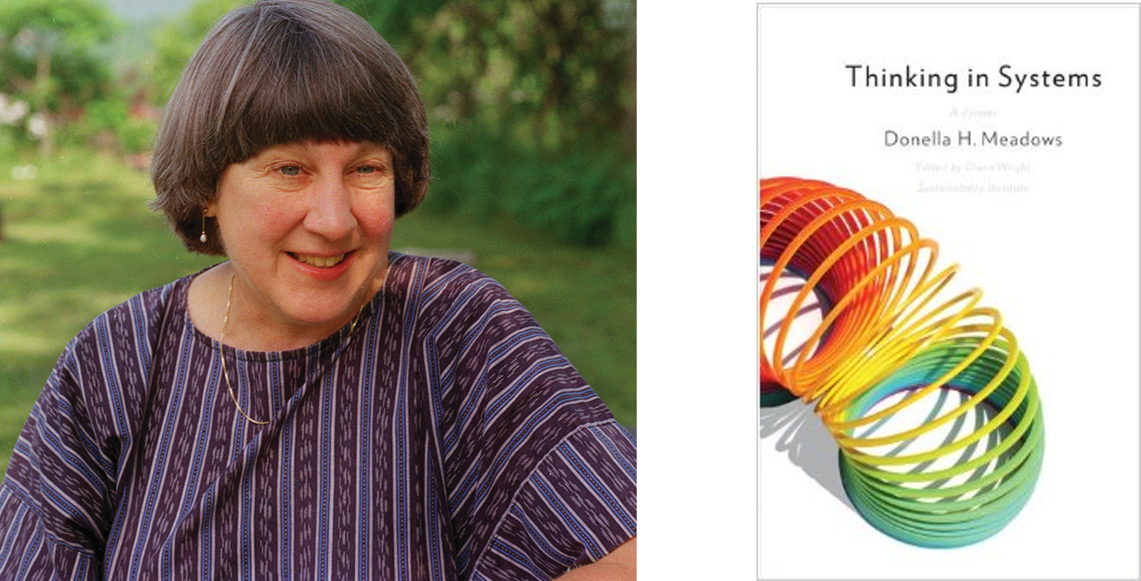
Figure 2.18: Dana Meadows (1941 - 2001)
The authors of the WORLD models saw some global problems, which could provoke the World Crises. These are overpopulation of our planet, lack of basic resources, critical level of pollution, food shortages, industrialisation and the related industrial growth. They tied a single variable to each of these issues. So, we have a six-level system, which define the structure of the WORLD model.
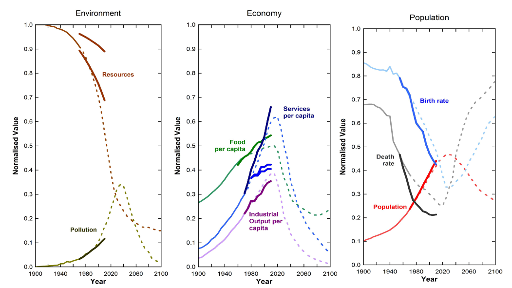
Figure 2.19: The ‘WORLD3’ model’s prediction of the future state of our world in the ‘business as usual’ scenario. Dotted lines: prediction of Meadows et al. (1972) and solid lines: observed data until 2010 (Turner and Graham, 2014)
The main descriptors for the status of our world seem to follow the predicted trends. Currently, we are in the plateau phase for most of these curves and start to witness downwards leading trends. Although not all predictions are accurate in their exact quantities and timing, the general trend is widely acknowledged today.
Book recommendation: Thinking in Systems (Meadows and Wright 2008)
In her research, Dana Meadows explored systems and their functioning in economy, ecology, the human body, the society, politics – in short all aspects of our everyday lives. Based on a broad knowledge and experience with system thinking she manages to provide an overview on general principles. And she was particularly gifted to explain these complex systems in simple words. The textbook “Thinking in Systems” (Meadows and Wright 2008) is an easy-to-read introduction to Systems Theory, which is based on Dana’s lecture notes. It is excellent and highly recommended reading, if you are caught by the ideas of system science and you want to dive deeper.
Last but not least, in case, you want to play around with the WORLD3 model yourself, you can find an implementation of it in Insightmaker:
Figure 2.20: Tragedy of the commons model, provided by Gene Bellinger