9 Model design
In the previous lessons you gathered knowledge on the fundamentals on systems theory, implemented your first spatial simulation models and explored how AI tools can support the development process. With increasing model complexity, designing a model carefully before writing a single line of code becomes essential. This is not a preliminary step, but the foundation everything else depends on.
By the end of this lesson, you will be able to:
- conceptualise a system to be able to represent it in a computer model for a given purpose by specifying the modelling approach, the spatial and temporal scale and extent, the elements (agents / cells) with their attributes, their behaviour, and the nature of their relations, as well as the environment,
- define input parameters, state variables to monitor the state of the modelled system, and a set of spatio-temporal validation patterns that can be quantitatively compared to observed patterns,
- formalise the conceptual model by means of a UML activity diagram,
- identify major sources of potential uncertainty due to simplifications and assumptions.
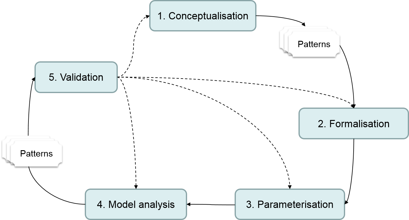
A conceptual model is the most fundamental level to describe and discuss a model. Its design specifies the system components, their interrelations, the temporal and spatial scale and the boundaries of the system, the input parameters, state variables, and expected outputs. In this initial phase the entire modelling cycle (Figure 9.1) is already in view: what is decided here determines what can be coded, what can be parameterised, and which patterns will be available for validation. Computers are not much needed. A lot can be done with pen and paper, and the work consists of building an understanding of the system structured deeply enough to be written down as rules. Not surprisingly, the most fundamental kinds of error and uncertainty are related to the conceptual model of the system.
Lesson 5 encourages AI-assisted coding, and this lesson asks you to design without it. Why?
Code can be wrong in a way you can detect, because the conceptual model is what you check it against. A conceptual model has nothing to be checked against, which is why this step stays with you. A model is a formalised hypothesis: if the hypothesis is not yours, a mismatch between model and reality tells you nothing, because none of your assumptions has been contradicted. The model still runs. It has simply stopped being an instrument of understanding.
9.1 Problem definition
It can be a quite daunting task to sit in front of an empty sheet of paper and having to start designing a model. To approach model design in a structured way, I recommend to always start with the purpose of the model: Why do you want to design a model? Which problem should it help to solve? What exactly is the question? Who wants to work with the model and who is interested in the outcomes of the simulation? What is the nature of the expected outcome, how accurate do the results have to be and how much uncertainty is acceptable?
Write down the problem definition in full sentences and be as specific as possible.
For those of you, who are experienced in academic writing, it may help to think about the modelling purpose like a research question: define an overall aim and then specify the operational objectives that you want to achieve. The problem definition will guide you through each step in the design process. Make sure to refer back to your problem definition for every design decision. As your modelling project grows, your understanding of the system and the nature of the problem will deepen, and you will most probably have to revise and refine the problem definition.
The deeper you will dig into the system that you want to model, the more details you will add to make the model more realistic. However, always have in mind: adding detail does not necessarily improve the model! There is a level of medium complexity beyond which it does not pay off to add further details. Models that are too complex lose their explanatory power, because the causality of relationships between the model structure and its emerging behaviour gets blurred. The below quote is often attributed to Albert Einstein. It says it all:
Models should be as simple as possible, but not simpler than that.
Modelling follows the principle of the so-called Occam’s razor: it states that among competing hypotheses, the one with the fewest assumptions should be selected. Other, more complicated models may be correct, but the fewer assumptions made, the better it generalisable and transferable to other study areas or use cases. With other words: simple is beautiful. A modeller will proudly describe his or her model as elegant, if it is very simple and still explains complex behaviour.
A strategy to finding the zone of medium complexity of a model between abstract simplicity and untraceable complexity that has proven successful in practice is the rapid prototyping approach. You quickly produce a simple prototype by reusing existing building blocks, parameterise it with plausible values and run a first simulation. After subsequent analysis and validation of the first results you will already have a good grasp on what the model does and what is still missing. Probably you need to re-conceptualise parts of the model, add code, refine parameters etc.: you are going to iterate through the ‘modelling cycle’ many times until the model is good enough for the purpose it is designed for.
9.2 Model specification cookbook
9.2.1 Modelling method
This is the time to double-check:
Can the problem definition be solved with an analytical approach, or do you really need to approach the question with a simulation model?
Only when you have positively answered this question, you can think about:
Which modelling approach is most adequate for the given purpose: a CA, an ABM, or another spatial simulation approach?
9.2.2 Entities and their properties
Next, define how to represent the active entities of your model:
Write down the list of agents and / or CA-cells that will be modelled.
Think about the properties that you want to represent for the agents, for the environment, and also for the entire system.
Define all relevant agent attributes, cell attributes and global attributes.
Note them down as well.
9.2.3 Spatial scale and extent
There are at least two spatial and temporal scales in a simulation model: the system-level scale and the individual-level scale.
First, the broader system-level scale needs to be set. For example, a model of the habitat expansion of an invasive frog species will probably look into the extent of the entire potential new habitat of the species.
Define the extent of the modelled study area.
Second, the finer individual-level scale at which the modelled elements operate. What is the spatial granularity of the model? In an agent-based model, this would be the local neighbourhood of individual frogs, in a cellular automaton it would be raster cells of potentially inhabitable wetland patches.
Define the cell resolution of a CA, and the typical distance of an agent’s neighbourhood for (inter)action
While the definition of the spatial scale at the individual-level seems to be straightforward at first sight, the decision on an adequate scale carries a lot of potential in terms of abstraction and simplification. Is it necessary to model each individual egg as an agent? A single frog can lay several hundreds of eggs, so this decision implies, whether the model needs to deal with millions rather than thousands of agents. Working with wetland cells in a Cellular Automaton instead of agents may reduce it further down to a few hundreds of cells. This decision of the spatial model granularity can imply that a simulation run takes a few seconds versus several hours (or crash completely).
Remember at this point the guiding principle for all design decisions: models should be as simple as possible, but not simpler than that. Models that just take a few seconds for a simulation run can be more fully explored, tested and optimised. However, the judgement on what is “necessary” in this context needs to be guided by the model purpose. If you are unsure, make a note about it, take the simpler case for now, and proceed.
9.2.4 Temporal scale and granularity
Closely linked with the spatial scale is the temporal scale:
At the system-level scale, the period of time covered by one simulation run sets the temporal extent of the model. It needs to be in an order of magnitude to capture the phenomenon of interest. For the frog example, it can be the period of habitat expansion since the species was introduced until today, and maybe also projected to the next 20 years.
Define the period of time covered by one simulation run.
To set the individual-level scale, we need to define the length of a time step. The granularity of time steps need to facilitate the representation of individual behaviour. Taking up again the example of the invasive frogs: single out the individual-level processes that are relevant for invasion into new territory. Is it necessary to explicitly model competition for resources between individual eggs in a pond? Probably not. Is it necessary to explicitly model frog migration from ponds to hibernation places and in spring further to (new) ponds? Probably yes. Do you want to model migration adaptively in response to land cover, weather, and other frogs, or is it enough to let the frog “jump” an assumed maximum migration distance? What does this decision mean in terms of adequate time steps? It can be anything between minutes and months.
Define the length of a time step.
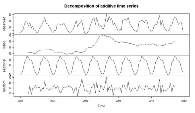
In difference to space, the temporal domain is uni-directional and cyclic in nature. Day-night patterns or seasonal oscillations lead to strongly self-similar properties of temporal phenomena. In temporal data analysis, we can utilise this property of time to decompose spatio-temporal patterns into multiple scales (see Figure 9.2).
9.2.5 Boundaries
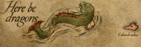
In simulation modelling there are several ways to handle these dangerous fields:
- The world ‘ends’ at the boundary
This is a pragmatic approach that is usually applied for real-world study areas. The open question is how to simulate local neighbourhoods beyond the borders. In cellular automata, the rows at the edge need to adapt their neighbourhood rules to the reduced number of actual neighbours. Agent-based models with moving agents often have a ‘bouncing’ algorithm, where the agent turns by 180° or where it bounces like a ball on a snooker board.
Do you expect any boundary effects that you want to mitigiate with a buffer area? Further, do you want to consider the world outside the modelled study area: e.g. is there any migration of agents from or to the outside, or is there any in-/outflow of matter?
- The world wraps
Wrapping worlds are often used in homogeneous (artificial) landscapes: an agent that leaves the scene on the left re-enters at the right side. It is a common approach in abstract, theoretic models. This never-ending concept of space is called toroidal (‘doughnut-like’) space.
Specify the type of spatial boundary (finite or toroidal).
- Temporal boundary: spin-up phase
What about temporal “boundary” effects: does you model need a spin-up phase to reach the state from which you want to actually monitor the simulation?
Specify, if a model spin-up phase is foreseen.
9.2.6 Process schedule
Many of the decisions on the spatial and temporal granularity of the model are linked to the processes that need to be modelled. Make a list of all involved processes and briefly describe each of them. For a CA model, processes are encoded in transition rules for a defined neighbourhood. The description thereof should be straightforward. To describe the behaviour of an agent can grow more complex. For a structured approach to describing agent processes, it is helpful to think about the conceptual decision-making frameworks that we have discussed in the lesson on Agent-based models.
List all relevant individual-level processes for each agent / CA, as well as globally operating processes.
The next task in the design process is to schedule the identified processes. Scheduling refers to the logical order of processes through which an agent or cell in a CA iterates in each time step. The execution order can strongly affect simulation results. For example, the amount of frog eggs in a pond depends on the order of the processes ‘old-frogs-die’ and ‘frogs-mate’. For some processes there is a clear, sequential order. Other processes depend on a condition, related to the state of the agent, of another nearby agent or of the local environment. Note down such conditions.
Connect the processes into a logical sequence, using conditions.
9.3 Validation patterns
Now, that you have specified all important aspects of your model, it is time to think about validation.
Which data are available to validate simulation outcomes? Can you simulate and quantify the same type of data that you have in mind for validation, so that you can compare these data sets statistically? Besides the main results that you expect from your model, which other simulated side-results could be used for quantitative comparison with observed data?
The more different aspects of the modelled system are available for comparison between the observed and the simulated world, the better you can validate your model.
9.4 UML activity diagram
Finally, you have to bring the model design into a structured format. To specify the conceptual model in a rigid way, we can make use of “diagrammatic modelling”. In this established approach from software engineering, conceptual models are sketched graphically in diagrams based on certain notation standards.
Several alternative graphical notation standards have been suggested for the specific purpose of agent-based modelling. Among the proposed notations is the Business Process Model and Notation (BMPN) (Onggo & Karpat, 2011), the Unified Modelling Language (UML) (Bersini, 2012), or adaptations of these standards such as Agent UML (Bauer et al., 2001), or the Agent Modelling Language (Červenka et al., 2004). The true power of all of these methods is that model diagrams can automatically be transferred into executable code. Unfortunately, the ABM community has not yet agreed which standard to use for declaring conceptual models. Nevertheless, software developers have started to implement graphical editors into ABM software environments, e.g. statecharts for Repast Symphony (Ozik et al., 2015), or the Graphical Editor for the GAMA modelling platform (Taillandier, 2014). The latter is built on UML class diagrams, which are excellent to capture the structure of a model (its agents, attributes and the environment), but are not well suited to represent the process dynamics. If you want to explore GAMA’s diagrammatic modelling option with UML class diagrams, install the Graphical Editor plugin. An additional integration of UML activity diagrams was planned (Taillandier, 2014), but unfortunately has not been implemented yet.
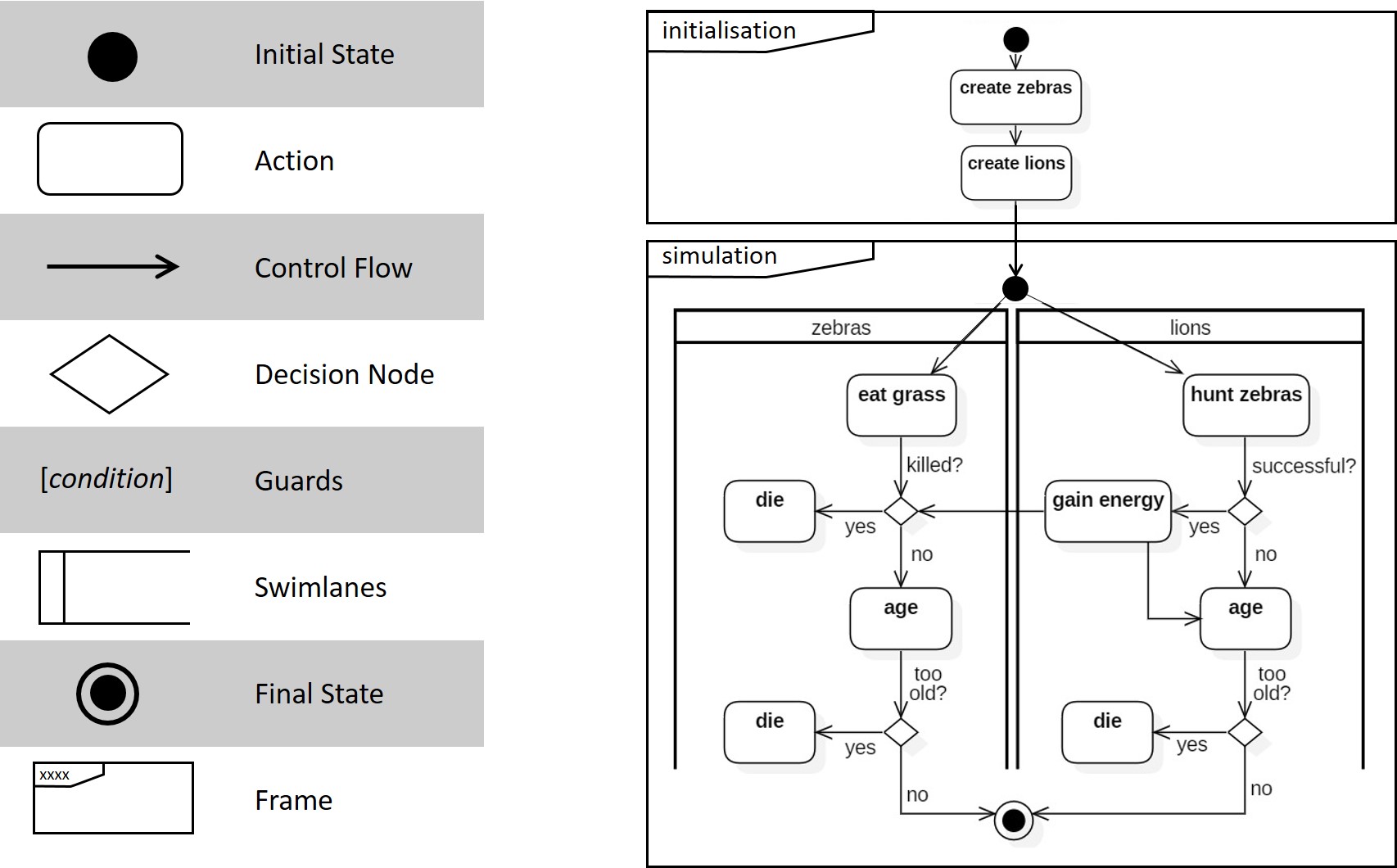
UML Activity Diagrams are particularly well-suited to capture (and communicate!) the logical flow of agent behaviour and interaction. Its UML notation is quite straightforward. For the purpose of capturing an agent-based model we need only eight symbols:
initial state This is the ONE node, at which the modelled process starts. A UML Activity Diagram can only have one starting node, unless there are several nested or encapsulated program parts. For the notation of an ABM model, it makes sense to separate the initialisation phase from the iterative simulation part. Each of these parts has its initial state node.
action The action (or activity) is the central element of a UML Activity Diagram. It represents the execution of an agent’s action or interaction, or an event in the environment.
control flow Control flows define, how the actions are scheduled. Control flows guide through the diagram and capture the logical flow of processes.
decision node Adaptive behaviour that follows rules with respect to the agent’s own state or the local state of the surrounding system are captured in decision nodes. Each single agent or cell decides individually at each time step. These individual, but potentially dependent decisions are responsible for the “smart”, adaptive behaviour, unpredictable, non-linear processes and ultimately emergent patterns at system level.
guards The outgoing control flow arrows from the decision node can be labelled with the respective conditions. These conditions are the “guards”, which make sure that only allowed agents may pass along this path.
swimlanes Swimlanes group related activities into one column (or one row). In ABM Activity Diagrams, swimlanes usually represent the pathway for one agent type or cellular automaton. This adds modularity to the Activity Diagram: it supports adding or removing agent types. Although swimlanes are optional elements, they usually give more clarity to an Activity Diagram and greatly help to keep a clear structure in the diagram.
final state The state which the system reaches at the end of the initialisation, or at the end of one simulation step is known as the final state. Once the final state of a simulation step is reached, the model is reiterated from the updated initial state.
frame A frame element in a UML diagram encapsulates sections of collaborating elements. For the purpose of representing an agent-based model, we can make use of frames to separate the initialisation phase from the iterative simulation part.
fork A fork node is needed, if from a certain point in time, there are two or more activity chains that happen in parallel. This is commonly needed, if there are several agent types and / or cellular automata.
In Figure 9.4, you can see the notation symbols of the UML Activity Diagram notation (left) and its examplary application to a predator-prey model (right).
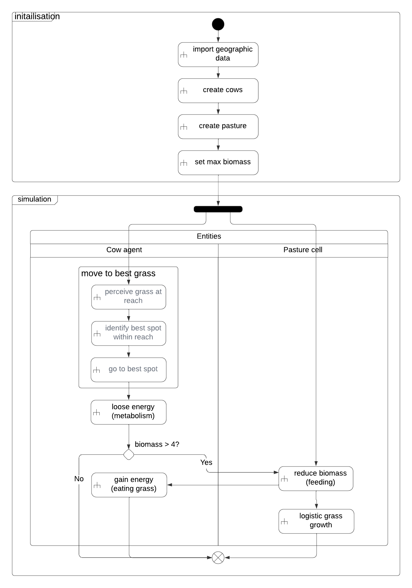
This exercise designs a model that does not exist yet. Take the Geosimulation pasture model from Section 4.3, in which cows wander over the pasture and grass grows, but the two never interact - and design the extension that makes them interact: cows feed on the grass, gain energy from it, and locally reduce the biomass.
Designing before implementing is the normal order, and it is why this lesson comes where it does. You will build exactly this model later, in Section 11.3.
The extension adds:
- a global variable for the range of the cows (their action radius),
- an agent variable for a cow’s energy level,
- an agent variable holding the grassland cells within reach,
- purposeful movement directed to the pasture cell within range that has the most grass,
- removing grass and gaining energy.
1) Software
There are several UML tools that you can use.
- Draw.io is the free online offer of a commercial product. You can use it without having to register. All shapes and functionalities that we need are there. It models UMLs in .xml format, so you can feed your diagram into an AI to have a structured starting point to develop your model. However, it doesn’t export a semantic UML (it doesn’t say “action node” but “rounded rectangle”), so you need a text that explains the semantics.
- PlantUML is a script-based UML tool. It fully encodes the semantics, but its visually not as pleasing as the other products.
- yEd, is a desktop application. It’s online version yEd live has a limited number of shapes (e.g. no swimlanes), and thus it can’t be used for the tasks.
- Lucidchart also is freemium online tool. It has a good usability with all features that you need, its look and feel is quite similar to draw.io. However, you have to register to use the software, and there are two further drawbacks: it is limited to about 60 objects in the free tier, and it can only export image files and thus is not very well suited as input into an AI-assisted implementation workflow.
2) UML design
Work your way from the general to the specific:
- start with the frames for initialisation and simulation,
- then add the swimlanes for the modelled entities (one lane for each agentset / CA)
- Add the init procedures
- Add the activities in the correct order to the swimlanes they belong to. In a well-designed code, you can think of each reflex to be an activity. However, sometimes activities can be organised hierarchically, i.e. a “super-activity” is a collection of a related set of small activities. It can make sense, to
- Connect the activities within one lane with control flows. If necessary, branch the flow through decision nodes. Label the guards of your decision nodes.
- Add the connections across swimlanes
- Add the start and the end node
- Make sure there are no circles or unwanted dead ends. Check all connections and follow the logic from the start node til the end node, taking the perspective of one of your agents / cells. Everything fine?
Done! If you want, you can check the solution in the drop down. But as always: have your own try first!
Figure 9.5 is a sample solution for a UML of the cattle-pasture model. Your UML diagram may differ, e.g. in the level of detail. However, the logical structure should be the same.
Two things to focus at:
- In the cow agents, there is a hierarchical activity: the aggregate activity “move to best grass” consists of 3 micro-activities.
- Do you have the same order of activities in the grassland CA?
9.5 ODD protocol
The ODD protocol is a formalised template to summarise the results of the design process for an agent-based model. It complements the more code-oriented UML diagram in that it makes the purpose and the conceptual foundations of the model explicit.
Agent-based models have received a lot of interest, but also considerable critique was formulated by the research community. A big share of this critique was addressed to the large part of subjectivity in the models that would limit scientific credibility. Descriptions of models varied strongly in their level of detail, lengthy verbal explanations with ad hoc structures made it difficult for readers to understand a model – and merely impossible to replicate it. In short, model communication was inefficient for both, the writers and the readers.
The reaction of the agent-based research community to this fair criticism was impressive: not less than 28 researchers came together to publish a joint paper with an agreed standard for the reporting of agent-based models (Grimm et al., 2006). The aim was to provide a framework of presenting a model in a way that ensures that any other modeller could rebuild a published agent-based model and replicate the results. This paper turned out to be highly influential. The suggested ODD protocol (Overview – Design – Details) was successfully adopted by modellers in the natural- as well as the social sciences as the standard way to report agent-based models in publications and on scientific model sharing platforms.
The elements of the ODD protocol are organised from the ‚big picture’ in the beginning to the details of the model in the end. It closely resembles the model design workflow presented in this lesson.
| Overview | Design concepts | Details |
|---|---|---|
| purpose, entities, state variables and scales, process overview and scheduling |
Basic principles, Emergence, Adaptation, Objectives, Learning, Prediction, Sensing, Interaction, Stochasticity, Collectives, Observation |
initialisation, input, submodels |
You have met the “overview” part of the ODD already in the model specification cookbook. This part structures the design and implementation workflow and also is a helpful guidelines of how to write a comprehensive model documentation.
Further, the ODD template provides a brilliant description and summary of the design principles of complex models that we have already met in Lesson 2. These design principles are very core do a model design, but they cannot be captured well by a UML activity diagram, so a structured, verbal description of these principles complements a UML.
Grimm et al. (2010, Supplement 2) proposed eleven design principles to describe the guiding theories underlying a model design in their ODD template for model documentation:
Basic principles
Which general concepts, theories, hypotheses, or modeling approaches are underlying the model’s design? Explain the relationship between these basic principles, the complexity expanded in this model, and the purpose of the study. How were they taken into account? Are they used at the level of submodels (e.g., decisions on land use, or foraging theory), or is their scope the system level (e.g., intermediate disturbance hypotheses)? Will the model provide insights about the basic principles themselves, i.e. their scope, their usefulness in real-world scenarios, validation, or modification (Grimm, 1999)? Does the model use new, or previously developed, theory for agent traits from which system dynamics emerge (e.g., ‘individual-based theory’ as described by Grimm and Railsback [2005; Grimm et al., 2005])?
Emergence
What key results or outputs of the model are modeled as emerging from the adaptive traits, or behaviors, of individuals? In other words, what model results are expected to vary in complex and perhaps unpredictable ways when particular characteristics of individuals or their environment change? Are there other results that are more tightly imposed by model rules and hence less dependent on what individuals do, and hence ‘built in’ rather than emergent results?
Adaptation
What adaptive traits do the individuals have? What rules do they have for making decisions or changing behavior in response to changes in themselves or their environment? Do these traits explicitly seek to increase some measure of individual success regarding its objectives (e.g., “move to the cell providing fastest growth rate”, where growth is assumed to be an indicator of success; see the next concept)? Or do they instead simply cause individuals to reproduce observed behaviors (e.g., “go uphill 70% of the time”) that are implicitly assumed to indirectly convey success or fitness?
Objectives
If adaptive traits explicitly act to increase some measure of the individual’s success at meeting some objective, what exactly is that objective and how is it measured? When individuals make decisions by ranking alternatives, what criteria do they use? Some synonyms for ‘objectives’ are ‘fitness’ for organisms assumed to have adaptive traits evolved to provide reproductive success, ‘utility’ for economic reward in social models or simply ‘success criteria’. (Note that the objective of such agents as members of a team, social insects, organisms e.g., leaves—of an organism, or cells in a tissue, may not refer to themselves but to the team, colony or organism of which they are a part.)
Learning
Many individuals or agents (but also organizations and institutions) change their adaptive traits over time as a consequence of their experience? If so, how?
Prediction
Prediction is fundamental to successful decision-making; if an agent’s adaptive traits or learning procedures are based on estimating future consequences of decisions, how do agents predict the future conditions (either environmental or internal) they will experience? If appropriate, what internal models are agents assumed to use to estimate future conditions or consequences of their decisions? What tacit or hidden predictions are implied in these internal model assumptions?
Sensing
What internal and environmental state variables are individuals assumed to sense and consider in their decisions? What state variables of which other individuals and entities can an individual perceive; for example, signals that another individual may intentionally or unintentionally send? Sensing is often assumed to be local, but can happen through networks or can even be assumed to be global (e.g., a forager on one site sensing the resource levels of all other sites it could move to). If agents sense each other through social networks, is the structure of the network imposed or emergent? Are the mechanisms by which agents obtain information modeled explicitly, or are individuals simply assumed to know these variables?
Interaction
What kinds of interactions among agents are assumed? Are there direct interactions in which individuals encounter and affect others, or are interactions indirect, e.g., via competition for a mediating resource? If the interactions involve communication, how are such communications represented?
Stochasticity
What processes are modeled by assuming they are random or partly random? Is stochasticity used, for example, to reproduce variability in processes for which it is unimportant to model the actual causes of the variability? Is it used to cause model events or behaviors to occur with a specified frequency?
Collectives
Do the individuals form or belong to aggregations that affect, and are affected by, the individuals? Such collectives can be an important intermediate level of organization in an ABM; examples include social groups, fish schools and bird flocks, and human networks and organizations. How are collectives represented? Is a particular collective an emergent property of the individuals, such as a flock of birds that assembles as a result of individual behaviors, or is the collective simply a definition by the modeler, such as the set of individuals with certain properties, defined as a separate kind of entity with its own state variables and traits?
Observation
What data are collected from the ABM for testing, understanding, and analyzing it, and how and when are they collected? Are all output data freely used, or are only certain data sampled and used, to imitate what can be observed in an empirical study (“Virtual Ecologist” approach; Zurell et al., 2010)?