4 Geosimulation
The previous lesson established what geosimulation is, and when it is the right choice for a problem. This lesson builds one. You will implement an agent-based model and a cellular automaton that both read real geospatial data, combine them into an integrated model of a cattle pasture, and meet the question that every spatial model has to answer: whether its entities update all at once, or one after another.
By the end of this lesson, you will be able to:
- implement an agent-based model that loads and works with geospatial data,
- implement a cellular automaton whose cells are initialised from spatial data,
- integrate both into a combined geosimulation model of a real study area,
- decide whether a process should be updated synchronously or asynchronously, and implement it accordingly.
4.1 Agent-based models
In Agent-based models, spatial patterns emerge from heterogeneous individuals that interact locally. Even if agents are located in homogeneous environments, the expected result of such models is a self-organised, spatial pattern. The classic example is the clustering behaviour of social animals, such as flocking birds or schooling fish. The same phenomenon can be observed in groups of pedestrians.
There is no need to define an abstract, system-level parameter like “birth-rate”. Instead, the actual behaviour is implemented in a mechanistic way: individual females meet at the same location and at the same time with a male to mate and to produce offspring. So, Agent-based modellers are programmers that tell the story of the system in a formalised way.
In this exercise, cows will move on a pasture, where the geometry of the pasture is loaded from a .geojson file. If you successfully implemented the Hello World model of Lesson 1, you are ready to model with geospatial data.
I have commented my code, so that another modeller, who reads the code can easily understand what the code does. This is good practice in programming: I highly recommend that you do the same. Don’t wait with code commenting until you’ve finished, but comment as you go.
And again: make sure that you set your indents correctly. A well-structured code is easier to understand and it is much easier to spot errors!
Prepare the model
- Download the .geojson file of the pasture “Vierkaseralm” near Salzburg. GAMA has a specific folder structure to make referencing geospatial data easier. If you look into your Gama Project, you will find a folder called
includes. Store the pasture file there. - Create a new model in which 5 cows walk around randomly.
Load the geospatial data into your model
- Load the geospatial data into a global variable of type “file”. Always use relative paths to access files, otherwise your model won’t run on someone else’s computer.
//Load polygon file
file pasture_file <- file("../includes/vierkaser.geojson");- When you work with geospatial data in GAMA, you always need to explicitely define the bounding box of your model and read it into the predefined global “shape” variable. The command to get the bounding box of a geometry is
envelope():
//Define the extent of the study area
geometry shape <- envelope(pasture_file);- Read the geometry of the pasture into a variable:
//read the geometry of the pasture file into a variable
geometry pasture_geom <- geometry(pasture_file);
Restrict the cows’ movement
- Set the built-in agent variable “location” to
any_location_inthe pasture, when you create the cows.
//create 5 cow agents that are located within the pasture
create cows number: 5 {
  location <- any_location_in (pasture_geom);
}- In the agent section, adjust the movement. The default units, when you work with geospatial data in GAMA are metres and seconds. A speed of 1 would thus be 1 m/s = 3.6 km/h. Let’s slow down the cows and set the speed to 0.5 m/s. You can also set a maximum turning amplitude. Let’s set it to 90 degrees. Finally, you want your cows to stay in the pasture. This can be done with the “bounds” facet.
//behaviour: movement
reflex moveAround {
  do wander amplitude: 90.0 speed: 10 #m/#s bounds:pasture_geom;
}
Visualise the cows and the pasture
- In the agent section, you need to think about the size of the cow. Remember, that the default unit is a metre. So a circle(1) would be a cow symbol of 1m radius. It will be hard to spot on a pasture that has an extent of 2 x 2km. Try to find a good size!
- In the experiment section, draw the geometry of the pasture. The layers are drawn in the order that you write them. So, first draw the pasture, then the cows. Otherwise the cows would be hidden.
//draw the geometry of the pasture
graphics "pasture_layer"{
  draw pasture_geom color: #green;
}
Done - we have a basic model. Before we use this model to play around a little bit with it, I share the full code. So that you can compare and continue with the exercise, if anything doesn’t work for you.
4.2 Cellular Automata
In Cellular Automata, physical, social or ecological processes emerge from heterogeneous landscapes. The size, the shape and the connectivity of a landscape greatly impacts geospatial processes such as floodings, range shifts, dispersal, and colonisation processes, diffusion of air pollution, spread of wild-fires, or land-use change. In Lesson 1, you got acquainted with constructing and visualising a Cellular Automaton with GAMA. In the following exercise we move on to build a geospatial CA.
This exercises complements the geospatial ABM of this lesson. It adds a grazeland-environment to the cow agents.
A Cellular Automaton can be created directly from raster data that is read into a global variable of type “file”. Possible formats are ASCII and GeoTiff. However, in this exercise we construct a grid from vector geometries.
Within the “Vierkaser” pasture property, there are only some regions with open grassland, whereas the rest of the pasture has been overgrown with shrubs and trees.
- The “study_area.geojson” is the bounding box of the Vierkaser property Download,
- the “vierkaser.geojson” is the fenced Vierkaser property Download,
- the “lower_pasture.geojson” is an area with well growing grass within the fenced area Download, and
- the “Hirschanger” pasture is of lower quality within the fenced area Download.
Download each of the files and copy them into your /includes folder. With the following code you can load the data into your model.
    //Load geospatial data
    file study_area_file <- file("../includes/study_area.geojson");
    //fenced area includes shrubs and grassland
    file fenced_area_file <- file("../includes/vierkaser.geojson");
    //high-quality pasture area
    file lower_pasture_file <- file("../includes/lower_pasture.geojson");
    //low-quality pasture area
    file hirschanger_file <- file("../includes/hirschanger.geojson");
Next, we need to set the shape geometry that defines the extent of the model and read the geometry from the vector files, like we have done it in the previous exercise.
Initialise the CA
When we set up (=initialise) the CA, we construct a grid with a cell size of 5m x 5m. Each of the cells has two attributes: the current biomass and the maximum potential biomass per cell with a default value of 0.
To initialise the model we want to set the maximum biomass for each of the pasture areas: the lower pasture can grow up to 10 units of biomass per cell, the Hirschanger has a maximum of 7. Everywhere else within the fence, there are shrubs and the grass biomass can’t grow beyond 1.
To do so, we need to implement a conditional structure (if / else) and we need to do a spatial overlay operation.
if and else
Conditional structures with “if” and “else” are very important in Geosimulation: they can encode behaviour.
IF a condition is true, do something
if <condition> {
  do something
}
ELSE (the condition above is false) and IF another condition is true, do something else
else if <condition> {
  do something else
}
ELSE (if nothing of the above is true), do yet another thing
else {
  do yet another thing
}
for example:
if biomass > 5 {
  write "yummieh";
}Spatial overlay
GAMA offers all relevant functions that we need to evaluate overlay. Have a look at the GAMA Documentation for spatial operators to find out, which spatial operators are available. You will see, it’s quite a few – next to simple distance operators (e.g. closest_to) you will probably recognise the classical topological relations: touches, covers, crosses, intersects, overlaps. Here lies a lot of the power of GAMA’s spatial functionality.
To evaluate, whether a particular cell in the CA grid overlaps the Hirschanger pasture, we could write:
if self overlaps(hirschanger_geom) {
  write "This is Hirschanger";
}
Of course, it is not only possible to evaluate overlay, but also to perform an overlay operation. A union operation for example is as simple as that:
//union_geom is the union of polygon_A and polygon_B
geometry union_geom <- polygon_A + polygon_B;Creating a CA from a raster file
You can create a Cellular Automaton directly from a raster file. The input data needs to be either in ESRI’s .asc or the .tif format, and you also should provide the epsg code (here it is Web Mercator, epsg 3857) to make sure the raster projected correctly.
In the grid section, you can then construct the CA directly from the raster file. It will read the raster’s cell values into a built-in grid variable that is called grid_value. As it is built-in, you don’t have to declare grid_value, but can use it right away. The below code, simply writes each of the cell values into the console:
global {
    //declare the raster import file
    file my_raster_data <- grid_file("../includes/some_raster.tif", 3857);
}

grid myCA file: my_raster_data {
  init {
    write grid_value;
  }
}Now, try to implement the code that sets the current and maximum biomass:
- Lower pasture: max_biomass = 10, and biomass = 2
- Hirschanger pasture: max_biomass = 7, and biomass = 2
- everywhere else within the fenced area: max_biomass = 1, and biomass = 1
Make the CA dynamic
Finally, we let the CA grow grass in a reflex. Add a reflex that increases the biomass of each cell at each time step. The logistic growth function makes sure that the grass can’t grow beyond its maximum, and the update_colour reflex updates the colour to visualise the biomass change in the simulation.
To avoid a division by zero, we also need to restrict this reflex to cells within the fenced area with a max_biomass > 0. This could be done by using an if-condition within the reflex, but alternatively and more efficiently also the when facet can be used:
    // let grass grow until its maximum potential
    reflex grow_grass when: max_biomass > 0 {
        //logistic growth: N + r*N*(1-N/K)
        biomass <- biomass + grass_growth_rate * biomass * (1 - biomass / max_biomass);
        color <- rgb([0, biomass * 15, 0]);
    }
Done. The Cellular Automaton model reads a geospatial pasture polygon and models grass growth on that pasture.
4.3 Combined Geosimulation model
We could now combine the Agent-based cow model and the dynamic grass growth of the Cellular Automaton to a spatially explicit cow-pasture model. Actually, such combination of ABM and CA is the rule rather than the exception. It is the combination of smart individuals interacting in and with a dynamic environment (Figure 4.1).
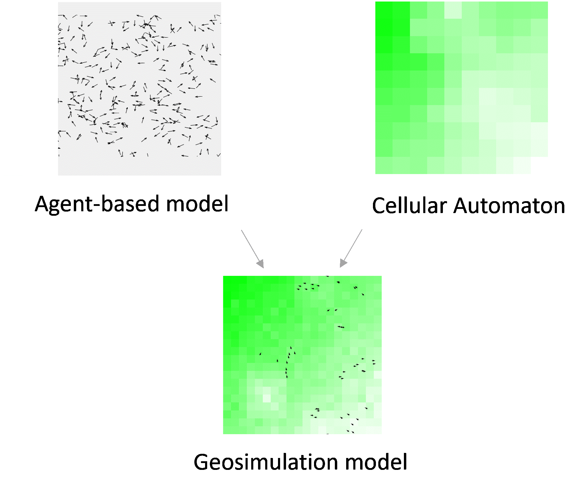
Another common representation of space is a network, e.g. for traffic simulation or for an abstract representation of topological relationships as for example in communication networks. Recent progress in the coupling of modelling frameworks with GIS enable advanced spatial data handling in agent-based models that to date were restricted to comparatively simple functionalities in terms of spatial analysis.
The next exercise of this lesson combines the two geospatial models of this lesson. Try to integrate the code yourself, before you look at the solution!
4.4 Asynchronous and synchronous update
Interacting agents and cells in a spatial model read the state of their neighbours and act according to their neighbours’ state. To model this process there is one important question: when does an entity update? Does it see its neighbours as they were at the start of the time step, or as they are right now — when some of them already have changed?
Both variations are valid. Whether asynchronous or synchronous updates are correct depends on the type of the process:
- Asynchronous. Each entity reads the current state and writes immediately, so entities computed later see the results of those computed earlier. Such asynchronous updates are typical for processes that compete for the same resource on a first-come-first-serve basis, for example citizens that look for an empty flat, cows that graze grass, or a lion mating a lioness. Biological processes are usually asynchronous.
In GAMA asynchronous updates execute the processes for cells or agents one at a time — one cell finishes all of its reflexes before the next cell starts. Reflexes within grid or species sections are therefore asynchronous by default. Two reflexes in the same grid are not two phases. Note the schedules: shuffle(my_CA) facet of the grid. This facet makes sure that the agents’ order is shuffled each time, which avoids artifacts that would emerge, if the process always executed in the order of the index.
For further reference, you can download the GAMA building block model “asynchronous update”.
model L4d_async_update

global {
    //reports final state of previous step
    reflex report_state {
        ask my_CA {write "" + self + ": " + CA_var;}
    }
}

grid my_CA width:2 height:2 neighbors:4 schedules: shuffle(my_CA){
    float CA_var <- 1.0;

    //take from neighbours
    reflex asynchronous_process {
        ask neighbors {
            float taken <- CA_var * 0.2;
            CA_var <- CA_var - taken;
            myself.CA_var <- myself.CA_var + taken;
        }
    }
}

experiment simulate type: gui {}- Synchronous. All entities read the same frozen state; the new values are written afterwards. No entity gains anything from being computed first. Synchronous updates represent processes where nothing is consumed, for example heat diffusion or water run-off. Physical processes are often synchronous.
In GAMA this is solved with a global ask that sweeps the whole population through one statement block before the next block begins. Two consecutive ask blocks in a global reflex divide the process in two phases, where a temporary variable is needed to freeze the state at the beginning of the time step.
For further reference, you can download the GAMA building block model “synchronous update”.
model L4e_sync_update

global {
    init {
        ask my_CA where (each.grid_x = 0 and each.grid_y = 0) {
            CA_var <- 5.0;
        }
    }

    reflex synchronous_process {
        ask my_CA { next_CA_var <- CA_var + 0.5 * ((neighbors mean_of (each.CA_var)) - CA_var); }
        ask my_CA { CA_var <- next_CA_var; }
    }

    //reports final state of current step
    reflex report_state {
        ask my_CA {write "final value from global sync process: " + CA_var;}
    }
}

grid my_CA width:2 height:2 neighbors:4 {
    float CA_var <- 1.0;
    float next_CA_var;
}

experiment simulate type: gui {}