2 Systems thinking and complexity
Simulation modelling rests on systems theory: the idea that a system is a group of interacting elements forming a whole that is more than the sum of its parts. That idea stands in stark contrast to conventional science built on Descartes’s reductionism, where understanding comes from breaking something down into its component parts (Cham & Johnson, 2007). This lesson works through both halves of the tradition. It begins with system dynamics - the first simulation modelling approach ever developed, and still influential across every domain - which describes a system through stocks, flows and feedback. It then turns to complexity theory, which asks what an aggregate description leaves out, and arrives at the properties that make spatial simulation necessary in the first place.
By the end of this lesson, you will be able to:
- describe a system through its three components: entities, connections and purpose,
- conceptualise a system with its stocks, flows and feedback loops in a stock and flow diagram,
- identify growth, decay, steady states and oscillation as the processes underlying system behaviour,
- distinguish a reductionist from a systems thinking perspective,
- characterise the properties of complex systems - emergence, self-organisation, non-linearity, path dependence - and explain why an aggregate model cannot reproduce them.
2.1 More than the sum..
A central aspect of the nature of a system can be sketched in a popular saying:
A system is greater than the sum of its parts
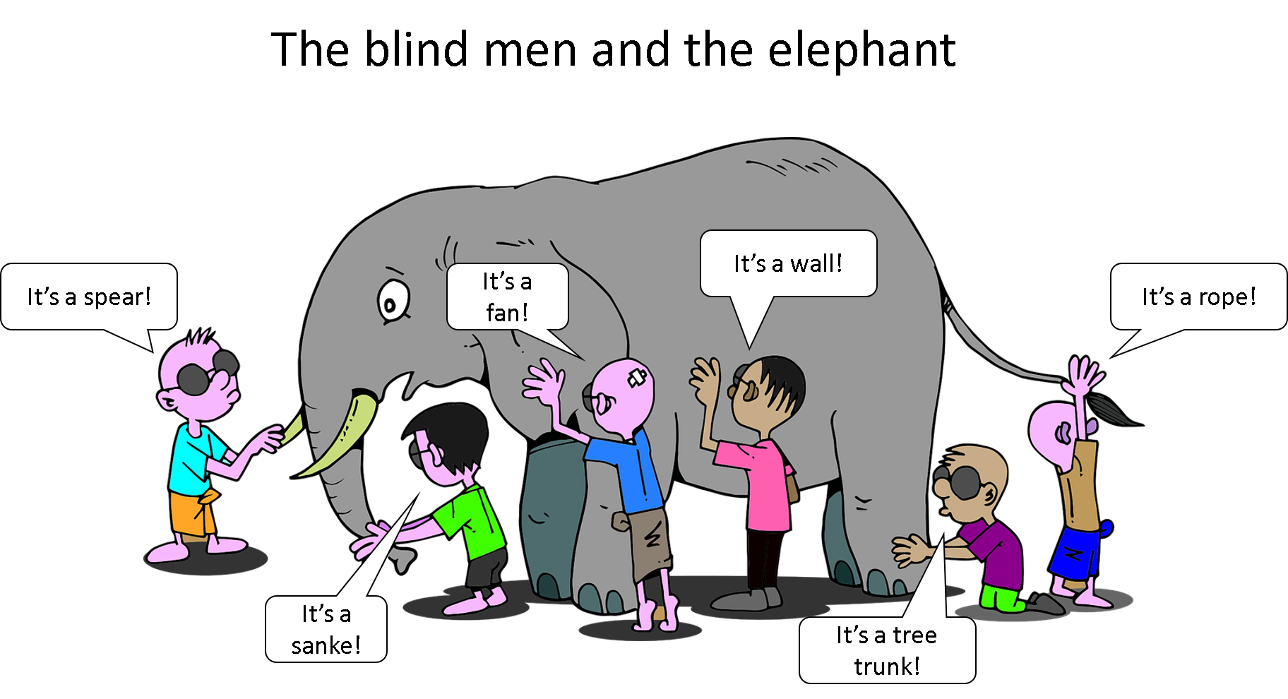
Traditional scientific approaches are focused on getting a better understanding of the world by ‘dissecting’ our complex environment into its parts and then establishing cause–effect relationships. Chemists and physicists dissected material into molecules, molecules into atoms, atoms into positrons and electrons and so forth. Accordingly, biologists tried to make sense of the environment by dissecting it to single species, and further to single animals, studying their individual behaviour and their physiology. This reductionist view of the world was juxtaposed by a holistic world view by system thinkers, who postulated that a system has a behaviour of its own and that such system behaviour can only be explained by studying the system as a whole. A population of animals behaves differently as we would expect from the behaviour of isolated animals. Just as a stock market follows rules of its own.
Let’s consider the hydrological cycle in an ecosystem. First, we are looking for internally homogenous parts of the ecosystem that are relevant in order to model the flow of water through the system. Each of these system elements holds a certain amount of water: clouds, snow, rivers, soil. The interrelation between the stocks is water that flows from one stock into another with a defined direction, e.g.: precipitation, snowmelt runoff, infiltration to groundwater, evaporation. We have now successfully designed a conceptual model of a system that has the function to perpetuate the flow of water through an ecosystem.
Another example is the human digestive system: It consists of different organs (stomach, intestine, liver, etc.) which are connected with the purpose of converting food into energy and waste.
These are two examples of ‘open systems’ in which we gain and lose material or energy in flows to the outside environment.
Both examples were built the same way: we looked for the parts, then for what connects them, and only then asked what the whole is for. Those three steps are not incidental - they are the components every system is made of.
2.2 System components
To be able to represent a system in a model, we need to have a conceptual understanding of the system; that is: we need to have a conceptual model. To come up with such conceptual model, it is helpful to think about the components of a system:
“A system is an interconnected set of elements that is coherently organized in a way that achieves something” (Meadows & Wright, 2008)
So, in short a system (and thus also a model of a system) consists of three components: 1) elements, 2) interconnections, and 3) a purpose or function. All three components are essential. If there was just an agglomeration of elements without connection and without purpose – for example a pile of sand – it would not be a system. When a living creature dies, it loses its ‘system-ness’. A football team can be viewed as a system: its elements are players, coach, field, and ball. Its interconnections are the rules of the game, the coach’s strategy, the players’ communications, and the laws of physics that govern the motions of the ball and the players. The purpose of the team is to win the game.
Elements are often the easiest part to conceptualise. A transportation system consists of streets, trucks, goods to be delivered, truck drivers, etc. An educational system is composed of a school or university campus, students, professors, etc. The football team would still function more or less the same way, even if we exchange each player. A university stays the same university, although generations of students pass through.
Interconnections hold everything together, they define the structure and the functioning of a system. What would happen, if we change the rules that a football must not be touched with feet, but only with hands? If students grade professors?
Changing its purpose affects a system most fundamentally. How would a football team function, that has the purpose to lose, instead of winning? How would a university look like that aims at persuading students of the ‘single truth’.
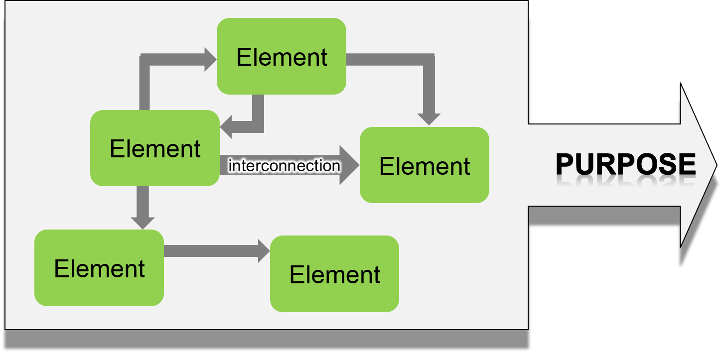
Elements, interconnections and purpose are what a system is. The next question is how to put them into a model that runs. System dynamics was the first answer to that question, and it remains the clearest: elements become stocks, interconnections become flows, and the purpose is what the modeller is trying to find out.
2.3 System dynamics modelling
2.3.1 Purpose
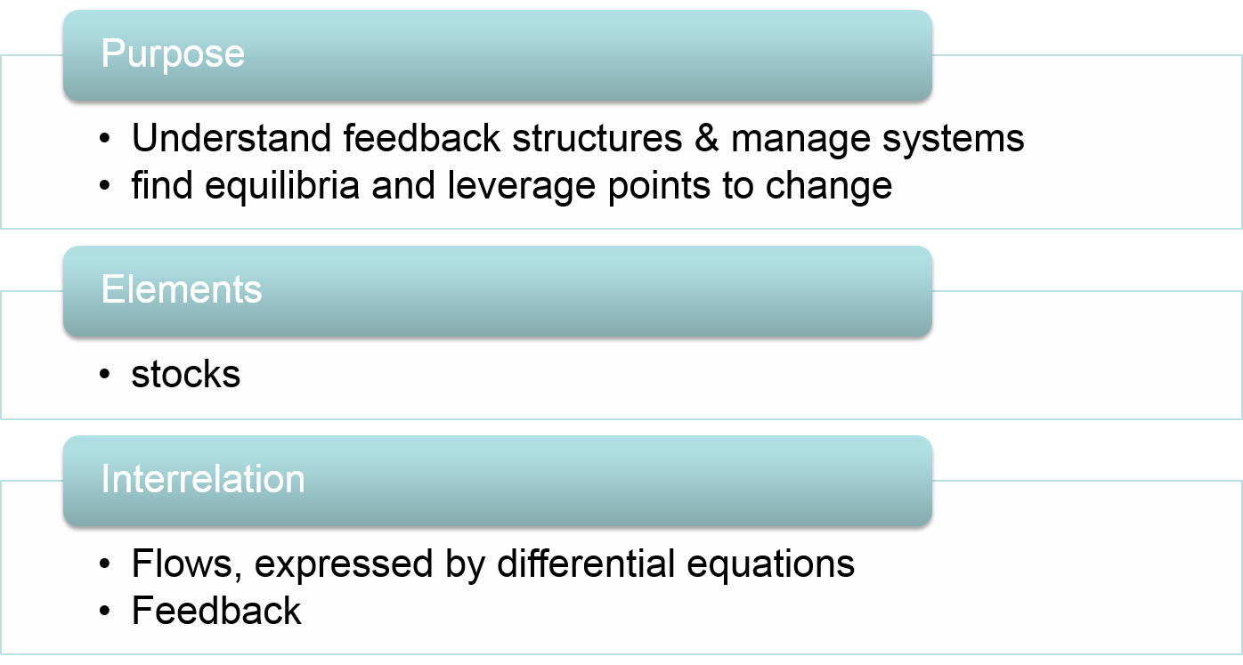
The purpose for which system dynamics was developed is to increase understanding of the dynamic behaviour of systems.
System dynamics is a mathematical simulation modelling approach with the core assumption that complex, non-linear behaviour of systems can be explained with a set of relatively simple processes that govern flows of energy and matter between interrelated, homogeneous sub-parts (stocks) of the system (Figure 2.3).
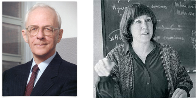
System Dynamics was developed by a group of researchers around Jay Forrester and Donella Meadows at the Massachusetts Institute of Technology (MIT) in the 1950s (Figure 2.4). In the absence of computers at that time, the scientists had to work with tedious hand simulations. Gladly, they took advantage of computers in the early days of this technical revolution.
2.3.2 Elements: stocks
Stocks are the core building blocks of system dynamics models. A stock is a homogeneous part of a system that holds a measurable amount of something in which we are interested – just like a container or system’s storage room. Examples for stocks are water in a lake, animals in a population, or money in a market. Stocks are easily recognised in a system and thus are a good starting point to conceptualise a system dynamics model.
Stocks by design assume average values across space. Although there have been attempts to tesselate space to some degree for designing spatial system dynamics models, the focus is given to dynamic patterns in the temporal domain.
However, the basic concepts of system dynamics are extremely helpful to understand models of complex systems. In this lesson, we will therefore explore some typical system dynamics models before we then move on to spatially explicit modelling approaches in the remainder of this module.
2.3.3 Relations: flows
Flows are ordinary differential equations that model, how stocks are linked together. Depending on the flow process, the stock grows or declines, oscillates or develops towards an equilibrium. Typical examples for flows are births and deaths, purchases and sales, growth and decay.
Let’s have a quick look at the maths behind flows: in ordinary differential equations, we describe how a variable evolves over time. These differential equations cannot be solved analytically. This means, there is no way to use mathematical methods to come up with an exact solution. Instead, we need to dissect time into small slices and calculate the linear difference between these time steps. So we turn a non-linear differential equation into small steps of linear difference equations. This stepwise approximation is referred to as the Euler method (Figure 2.5).
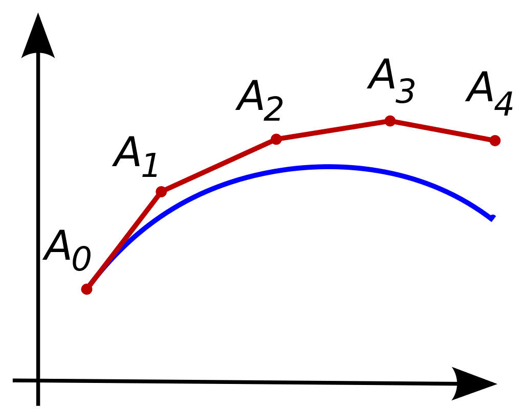
The Euler method takes an initial value from where it starts to solve the first difference equation. Taking the result it then iteratively solves the next equation, and the next, and the next, etc. This mathematical approach is called numerical simulation. The smaller the time steps, the more accurate is the result. System Dynamics software thus is a tool for numerical simulation of ordinary differential equations.
2.3.4 Stock and Flow diagram
A major asset of System Dynamics modelling software besides solving the ordinary differential flow equations with numerical simulation is the use of declarative modelling environments. These environments enable a modeller to use graphical representations of the system rather than writing equations and programming code. This convenient way of representing a system in a computer-readable form is termed ‘Stock and Flow diagram’. Figure 2.6 shows the notation rules to design a stock and flow diagram.
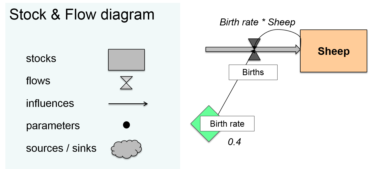
- Stocks
- Flows
- Influences show causal relations: which parameters / stocks influence a flow.
- Parameters quantify the ‘valves’ of a flow. Flows can increase or decrease – depending on the rate of change. By ‘turning the valves’ we manipulate flows.
- Sources and sinks represent the boundaries to the environment around a system. As we work in open systems, there is always an ‘outside environment’ that functions as source and/or sink.
2.3.5 Feedbacks
Feedback loops the key mechanisms to govern system behaviour. There are two types of feedback, reinforcing feedback accelerates and self-regulating feedback balances a system.
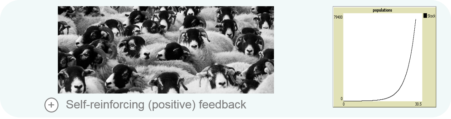
In the first case, we have a system with one feedback loop, which is a self-reinforcing (positive) feedback (Figure 2.7). It has positive causal links of the form ‘the more – the more’: the more sheep, the more lambs are born. The more lambs, the larger the population. The result represents the deregulated behaviour of a system: the population grows exponentially. An example for this dynamic behaviour are bacteria that are cultivated on an agar plate. Under good environmental conditions, bacteria are immortal. As long as these bacteria are not limited by the availability of nutrients, the growth dynamics is exponential. However, a self-reinforcing feedback can equally well have negative causal links of the form ‘the less – the less’, resulting in an exponential decay.
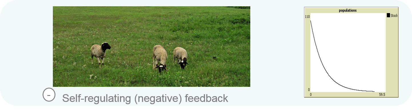
In the second case, we also have only one feedback loop. This time it is a self-regulating (negative) feedback (Figure 2.8). The result is a stabilisation of the population at a certain level: the population decreases proportional to its current value. The dynamics takes the form of an exponential decay. In this case, without any inflow, the sheep population approaches zero.
2.4 System behaviour
System dynamics model are very well suited to study the elementary ways in which a system can behave: linear growth, exponential growth, logistic growth, equilibrium (or: steady states) and oscillations (Figure 2.9). These processes govern systems and you will encounter them in all systems, regardless of the domain or the type of application.
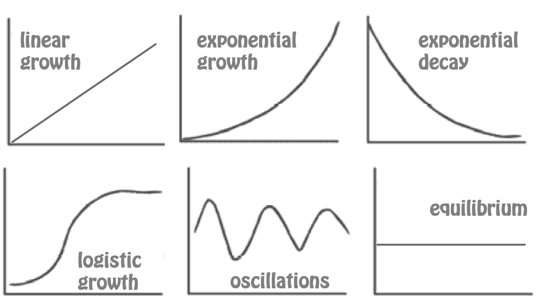
More complex system behaviour is always a combination of these simple process types. When we take multiple ‘simple’ concurrent flows to connected multiple stocks in a system, the resulting system behaviour will quickly grow to a complex, non-linear behaviour. However, these process types are not limited to system dynamics modelling. Later, when we turn to Geosimulation of spatial systems, you will observe, how growth, oscillations and steady states emerge from the local interaction between individuals.
2.4.1 Growth and decay
Linear growth or linear decrease results from constant inflow or outflow that is not related to the amount of the stock. An example would be migration. Mathematically, linear growth is described as follows:
Pt+1 = Pt + dt
The amount of P in the next time step will be the current amount of P plus the difference per time step.
In GAMA, you would simply write:
// P increases by x each time step
P <- P + x;
Exponential growth or exponential decay results from inflows or outflows that depend on the amount of the stock. We have encountered these processes in relation to feedback: self-reinforcing feedback always leads to exponential growth, whereas balancing feedback results in exponential decay. Mathematically, exponential growth is described with a stepwise approximation of diffential equations with difference equations.
Pt+1 = Pt + r * Pt
The amount of P in the next time step will be the current amount of P multiplied by the rate at which P grows each time step. Growth rates above zero result in exponential growth and rates below zero result in exponential decay.
In GAMA, you would write:
// P increases with the growth rate r
P <- P + r * P;
Logistic growth or logistic decay results from inflows or outflows that depend on the amount of the stock AND the carrying capacity of a system. Logistic growth starts off just like exponential growth, but the closer the state of the system approaches its carrying capacity, the more is the growth slowed down until it reaches a steady state. Mathematically, logistic growth is described with a stepwise approximation of differential equations with difference equations.
Pt+1 = Pt + r * Pt * (1 - Pt / K)
The amount of P in the next time step will be the current amount of P multiplied by the rate at which P grows each time step (=exponential growth) multiplied by the following clause: 1 minus the quotient of the current amount of P and the carrying capacity K. The latter clause approximates zero the closer P gets to the carrying capacity, and consequently Pt+1 cannot grow beyond K.
In GAMA, you write:
// P increases with the growth rate r
P <- P + r * P * (1 - P/K);
2.4.2 Equilibrium
Each living system has its own steady state in which internal conditions are stable and remain constant within amazingly narrow boundaries. For example, the temperature of a human body usually is just a little lower than 37°C. If this temperature rises by just a few tenths of a degree, we feel uncomfortable. If our body temperature is three to four degrees off, we are seriously ill. This tight temperature regulation works, no matter whether the air temperature around us is at +40°C or at -10°C. The same stable balance holds true for the levels of glucose in our blood, the calcium levels, and the blood’s pH. This very stable steady state in the physiology and metabolism of living organisms is called Homeostasis (from Greek for ‘similar state’). Only, if we expose ourselves too long in extreme conditions, our body cannot keep the balance and the system eventually collapses.
Figure 2.10 shows different types of equilibria. Homeostasis is an example for a stable equilibrium that is caused by balancing feedback loops, which push a system to progress towards its equilibrium and to get back to this equilibrium after disturbance (stable equilibrium). Whereas, dynamic equilibria are a special case, that are rare in real systems: inflows and outflows need to be at the exact same rate. If there is just a small imbalance, the system will develop in the one or the other direction.
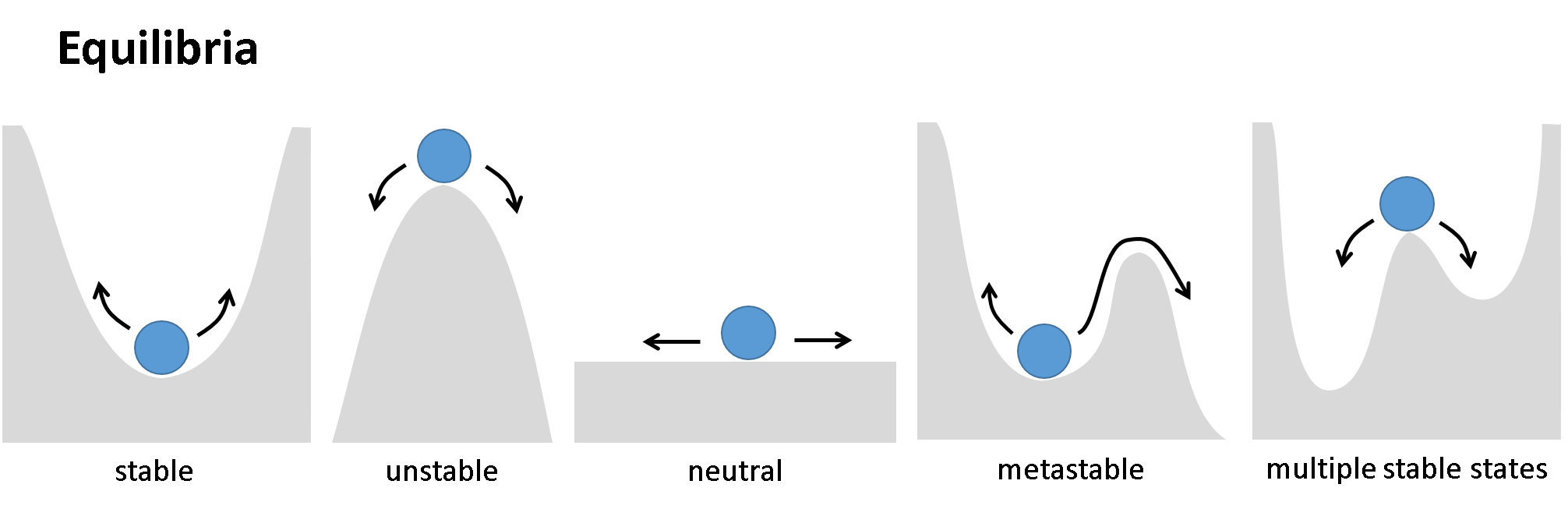
Systems theory starts from the premise that this phenomenon of stable steady states is also inherent to living systems at higher organisational levels, i.e. populations and ecosystems. As long as nature is in balance, an ecosystem will tightly control the flows of material and energy and its stocks will be balanced at a certain level. The steady state of a population that can be sustained by the resources in a certain ecosystem is called the carrying capacity of this ecosystem.
If a disturbance event results in an ‘unsustainable’ number of animals or humans in that population, the ecosystem has the capacity of regulating itself and recover its balance (resilience). However, if the disturbance exceeds a certain limit, the ecosystem collapses. The balance of nature paradigm has been under debate (e.g. Wu & Loucks, 1995), as things are always evolving and developing - not just since we witness climate change. Steady states are thus helpful to conceptualise a system, but in practice systems are rarely in steady states. Today, the concept is complemented with more bottom-up process oriented views related to complexity theory.
2.4.3 Oscillations
Last but not least, we look into oscillations. Oscillations in a system can have two causes:
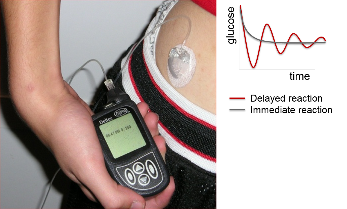
Oscillations by delay. Such oscillations can be seen, even if there is just one stock involved. An example are dangerous glucose levels after delayed insulin injections in diabetes patients (Figure 2.11). Similar oscillations can be found for delayed feedback reactions in all systems that are governed by balancing feedback loops, e.g. delayed orders and deliveries after an increased sales rate of a particular product; delayed reaction to changing temperatures in furnace systems; delayed reactions of a hunter to control a resource-limited deer population.
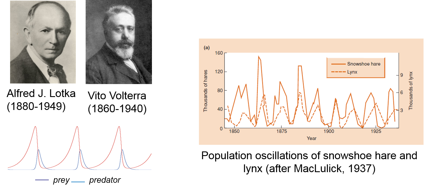
Oscillations by two interacting stocks. An example are disease outbreaks, in systems of interacting viruses and humans - we have seen this a lot during the Corona pandemic. Probably the most famous example of a two-stock, oscillating system is the predator-prey model. It was first formulated independently by two scientists in the mid 1920s. First, Alfred Lotka, who’s work was very influential to the academic world, although he followed a non-academic career and worked as a statistician at the Metropolitan Life Insurance Company most of his life. Second, Vito Volterra an Italian mathematician, who wondered about the oscillations of the availability of certain fish species in the Roman fish markets. The equations are today known as the Lotka-Volterra model. It is one of the most cited model in Ecology and it has inspired generation of researchers. The theoretical relation between a predator and a prey population has been proved empirically for many systems since, for example the abundance of snowshoe hare (Lepus americanus) and lynx (Lynx canadensis) pelts traded with Hudson Bay Company (Figure 2.12).
2.5 Implications of Systems Thinking
Following from system theory, a system is governed by its internal state, its stocks and flows, rather than by outside forces. Take a moment to think about the implications of viewing the world through the “system lens”:
- Bark beetle invasions do not damage forests. It is the single-species, same-aged forest structure optimised for the timber industry that facilitates the damage.
- Political leaders do not cause economic booms or recessions. Ups and downs are inherent in the structure of the market economy.
- The flu virus does not attack you. The overworked guy in Figure 2.13 may just set up the conditions for a virus to flourish within his body.
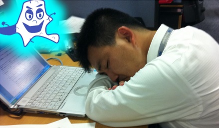
Psychologically, it is often easier to assume that a problem is ‘out there’ rather than ‘in here’. We would like to have a ‘control knob’ to solve a problem and blame somebody or something for causing a problem: flu viruses, bark beetles or politicians. Systems theory teaches us that things are not that simple and that we have to think differently, if we want to understand – and manage – systems.
Let’s have a look into some archetypical examples for the behaviour of (simple) systems from the perspective of Systems Theory. Well known system archetypes are Limits to Growth, Tragedy of the Commons, Eroding Goals, Shifting the Burden, Success to the Successful, or Escalation. You will find an Insight Maker model showcasing each of these archetypes. Here, we will look at two of them: Limits to Growth and the Tragedy of the Commons. There is a story to each model explaining the functionalities of the models. So just go ahead and click on the ‘Start Story’ on the bottom left.
Insight Maker online modelling tool
Insight Maker is free online platform for creating models and simulations. It allows users to create system models and share them online with others. You just have to create a profile and can start modelling. Insight Maker works mainly with drag and drop objects which you can alter and adapt. So it is easy to use and does not require you to know how to code.
2.5.1 Limits to Growth
Let’s start with the “limits to growth” system archetype (Figure 2.14). On the left side, there is a reinforcing feedback process that causes exponential growth. However, on the right side the system is balanced out by a negative feedback loop. The halt of the growth is imposed by limited resources: a commonly encountered system that keeps a stock within its limits.
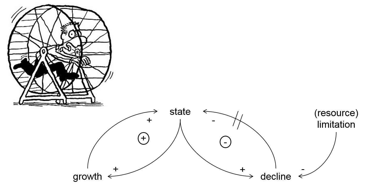
Sometimes we want to go beyond these ‘natural’ limits. We want to run faster and faster to win that competition. We want to produce more and more corn on the same piece of land. We expect better and better performance of an employee. However, as we fail to properly acknowledged the limits of a system, we have to push it harder and harder. The former methods are continuously applied, but more and more aggressively. Most of the effort vanishes through the self-regulating feedback loop on the right.
Explore the interactive Limits to Growth model in Insightmaker (Figure 2.15). You can think of agricultural food production as an example for this model.
Can the limitation be overcome? Think about what may happen, if you do so? Run a simulation with the default values and then try out to push the limits by dragging the limiting-factor slider from 20 to 50. Simulate again and compare the results.
2.5.2 Tragedy of the commons
The last system that we will discuss in this lesson is known as the „Tragedy of the commons”. The ‚commons’ are community-shared goods, for example a piece of land that belongs to the aggregate members of a community instead of an individual land owner. Let’s consider two farmers, who let their cattle graze on the commons. The more cattle farmer A sends to the commons, the more he will gain. The same is true for farmer B. The total amount of cattle of all farmers in the community is the ‚total activity’ on the commons. If there was no resource limitation, everything would be fine. However, due to limited resources there is a negative relation between ‚total activity’ and ‚gain per individual activity’. The more cattle are on the commons, the less grass is there for each single animal and the gain per animal diminishes. Unfortunately, until the agricultural land collapses completely the individual farmer still gains more the more cattle he has on the commons.
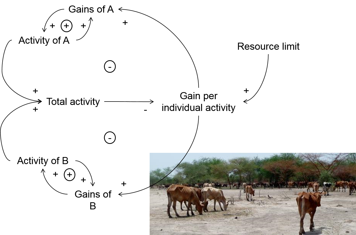
Many communities therefore put regulations into place, when and how the commons can be used by a member of the community in order to avoid a system collapse. A prominent example is the strict set of rules on the use of irrigation water in dry areas.
Notice what the tragedy of the commons needs in order to happen: herders who each decide for themselves, and who cannot see the consequences of everyone else’s decisions. A model that represents the herd as one aggregate stock cannot produce it, because the overgrazing arises precisely from the herders being separate. This is where aggregate thinking reaches its limit, and where a second tradition begins.
2.6 Complex systems
Weaver (1948) offered an interesting view on complexity. He argued that classical science traditionally has focused on systems with either just a few or a great number of elements. In the first case problems can be solved analytically (i.e. with mathematical equations), latter problems can be treated with statistical methods. Unfortunately, in the real world we often find ‘middle-numbered’ systems between these two extremes with too many unknown variables for an analytical solution and at the same time not enough to average out. Single events in such complex systems can have large impact on the results and outcomes are hard to predict.
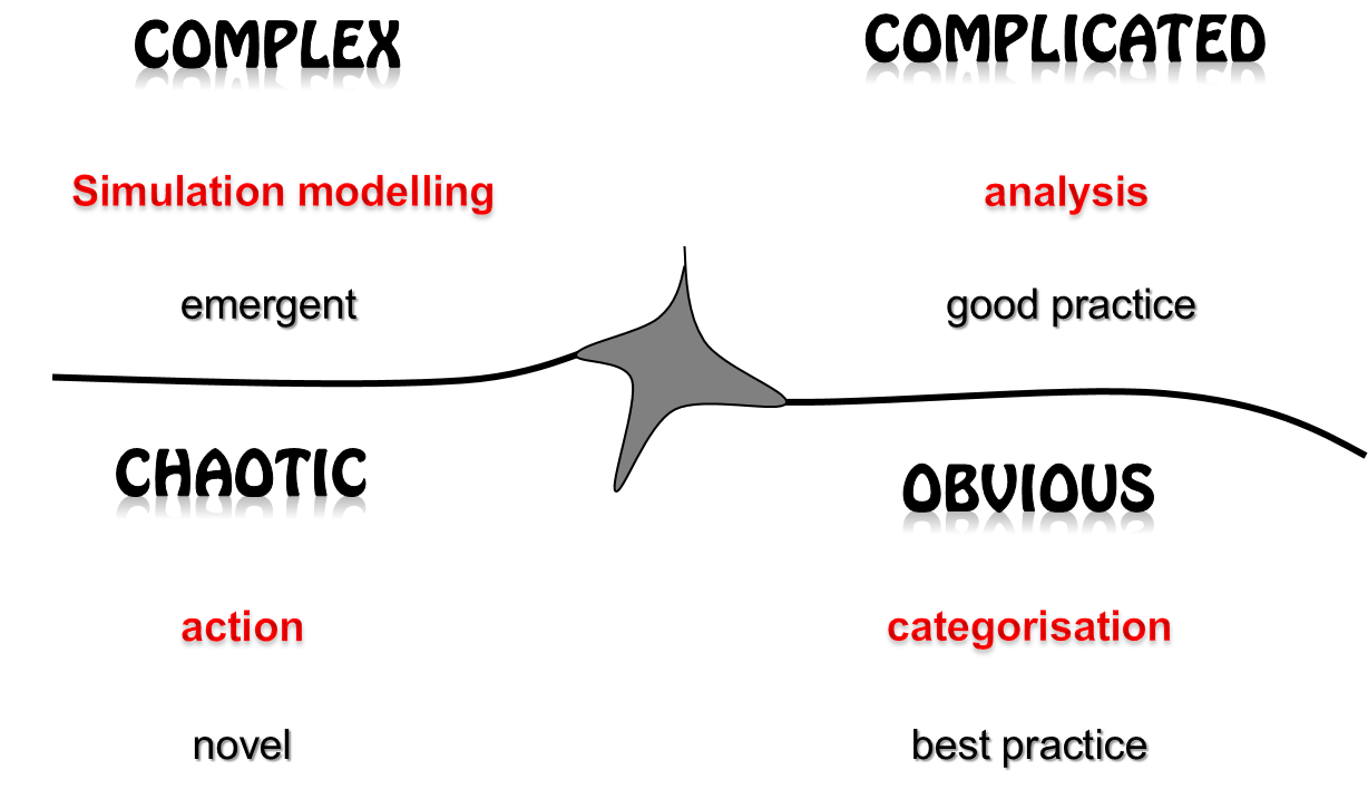
Along these lines, decision making situations can be categorised into four problem domains that afford different solution strategies - known as the ‘Cynefin (kʌnɨvɪn) framework’ (Snowden, 2000):
Simple problems can be solved by straightforward categorisation; there is a clear ‘best practice’ solution
Complicated problems need to be analysed to find an adequate solution. The solution represents ‘good practice’ (there might be other good solution too)
Complex systems follow some guiding principles, but the behaviour of the system cannot be intuitively predicted: it ‘emerges’ from the behaviour of system components. This problem domain lends itself for simulation modelling as tool that helps solving problems.
Chaotic systems have no inherent causal relationships, every situation is novel and the first solution strategy is immediate action to stabilise the system.
2.7 Complexity Theory
What would happen, if a bunch of the brightest scientists of the time from domains as different as physics, economy and computer science came together for a workshop to define the essence of what they all feel to be an emerging new approach in science? What if there were enough funds to found a research institute without any departmental boundaries to offer these researchers a place to collaborate and develop their ideas further? The result would probably be a promising new way of thinking – a new theory that brings about a paradigmatic change.
This is in short the story of the Santa Fe Institute in New Mexico and how Complexity Theory was developed. Shaping Complexity Theory has been a collaborative endeavour. However, if I was to name one ‘father’ of complexity this would most likely be John Holland, who published the Theory of Complex Adaptive Systems (Holland, 1992).
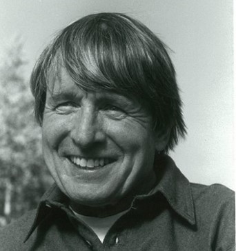
Here is an excerpt from Santa Fe’s website (http://www.santafe.edu):
In 1975, Holland published the groundbreaking book Adaptation in Natural and Artificial Systems, which has been cited more than 50,000 times. Intended to be the foundation for a general theory of adaptation, this book introduced genetic algorithms as a mathematical idealization that Holland used to develop his theory of schemata in adaptive systems. Later, genetic algorithms became widely used as an optimization and search method in computer science.
Complexity Theory is a systems theory just like system dynamics. It builds on the assumption that the whole is more than the sum of its parts. Complexity Theory also conceptualises the structure of systems to be made of elements that are connected together. It proposes that systems are non linear, so that small catalysts can cause large changes and that systems are self-organising. However, in difference to system dynamics, which describes a system from the top down through aggregate stocks and flows, it works bottom-up, with interacting individuals as its basic elements.
In the geospatial domain, complex systems are of particular interest, because local spatial configuration provides the structure for interactions between individual entities in the system. Whereas traditional simulation modelling approaches that rooted in systems theory chiefly were concerned with non-spatial temporal progression, complexity theory is equally concerned with both, time and space (O’Sullivan, 2004).
In the following, the main characteristics of complex systems are presented and exemplified with interactive toy models. The software to show these models is NetLogo Web, the browser-based version of NetLogo, which is a popular programming environment to develop agent-based models. This open-source software is authored by Uri Wilensky and it is widely used by the modelling community to develop agent-based models and cellular automata. You can explore and even modify NetLogo models online through NetLogo Web.
2.7.1 Individuals are unique
Central to the philosophy of complexity is that no individual is like the other. Each member of a population differs from its mates or peers in sex, age, size or colour. More profoundly it also differs in memory, experience and behaviour. Between some individuals there are stronger social bounds than between others. Not least from a geographic perspective individuals differ by location. Even if all individuals were the same, these individuals would differ by their spatial context: one would be closer to a food source, or more in the centre of the protecting crowd, or it would occupy a superior nesting site.
The richer the behavioural variety of a species, the stronger will individuals differ and the less suited are general system models that are based on differential equations of “stocks” and thus assume that the individuals in a system are all equal. A striking example of this concept was published in the influential, first review paper on Agent-based models in the Ecological domain by Huston et al. (1988): Figure 2.20 shows that a general system model with equal individuals completely differs from a complex system that consists of unique, spatial individuals.
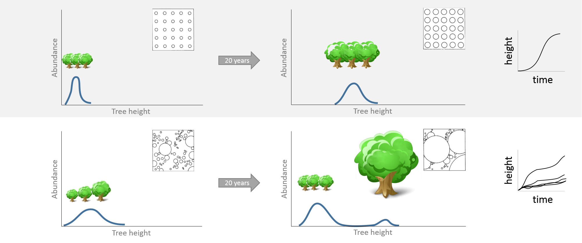
Figure 2.21 is an interactive model that reproduces the results published by Huston et al. (1988).
To initialise the model, press the setup button and to run the simulation, click go. You can see the tree biomass histogram bar move from left to right, as the forest grows. Now, check the “spatial” box, setup the model again and run it. Can you explain, why the model results in a bimodal distribution in the histogram of tree biomass? Or in other words: why are there just few big trees and so many small trees?
2.7.2 Individuals adapt
An individual’s ability to adapt is the second fundamental difference between conventional and complex systems after heterogeneity of individuals. Such capability can be encoded in behavioural rules, but it is not mathematically tractable.
Adaptation can refer to immediate response to a situation, or it can initiate learning processes that may manifest in later actions, or it can trigger long-term evolution through genetic exchange, mutation and selection.
Figure 2.22 shows the model of a famous example for genetic evolution in response to environmental change. Due to severe air pollution following the industrial revolution, white birch trees near Manchester, England, turned black. For a specific white-coloured moth species this turned out to be a real problem, because suddenly birds could easily spot them, and the number of Biston popularia (peppered moth) declined drastically. However, after some generations, mutations of darker morphs appeared and the population survived.
Again, click on setup and then on go to run the peppered moths model. While the simulation runs, pollute (click the button several times) the environment. Can you see, how the moth population adapts to the darker colour, because well-adapted individuals have a higher survival probability?
2.7.3 Emergence
The unique characteristic of complex systems is emergence: the non-intuitive formation of system-level patterns from the interaction of individuals with their neighbours and the local environment. It is the contrary to top-down imposed behaviour. Emergence is rooted in the structure of a complex system, which is defined by the connections between individual entities (remember the social theory of Luhman: communication links are more important for a society than individual persons). Thus, the interactions between entities lead to the emergence of complex system patterns such as bee hives, schools of fish, commuting patterns and social communities.
If there is a specific set of links and interactions types between individuals (such as the social behaviour of bees), similar systems (bee colonies) will emerge. Also for the much richer human behaviour, similar system patterns emerge in a largely self-organised way: urban street networks, communication clusters or food supply chains.
Grimm and Railsback (2013) identify three criteria of emergent behaviour:
- Emergent properties are not simply the sum of the properties of the individuals
- Emergent properties are of a different type than the properties of the individuals (e.g. the spatial distribution of individuals is a system property of a type that none of the system’s individuals has)
- Emergent properties are often counterintuitive and cannot easily be predicted by looking only at the individuals.
To better understand the concept of emergence, which is central to systems thinking and modelling, take a cup of tea and watch the video below (Figure 2.23). It explains the concept with nice visualisations and a couple of examples.
A strikingly simple and yet fascinating example of emergent patterns is the generation of clustered movement (“flocking”) in social animals. Let’s explore it further in the following exercise.
Now, explore emerging patterns yourself by playing around with the flocking model (Figure 2.24). The model is based on the work by Reynolds (1987) and it has been implemented in NetLogo Web.
The flocking model has five parameters. Move the individual sliders and you will immediately see how the birds’ behaviour changes. Can you find a parameter setting, in which the flock does not move forward into any direction, but just builds a stationary flock, like midges sometimes do, when they dance around themselves?
2.7.4 Self-similarity
Complex systems emerge from iterative processes. As a result, the emerging patterns often repeat themselves at different levels of scale: when we paddle up a river we will see it bifurcate repeatedly until we reach the spring. Analogously, informal settlements consist of shelters, which are part of a block, which in turn is part of a quarter – an emergent pattern that was not planned by any city government. The same is true for coast lines, trees, ferns or ice crystals. An almost perfect example for a natural self-similar pattern is the Romanesque Broccoli.
The hierarchical structure of self similar systems can be described mathematically as fractals. The idea of fractal dimensions was pioneered by Benoit Mandelbrot. The fractal dimension is a ratio that provides a statistical index of complexity: it compares how the detail in a pattern changes with scale at which it is measured. This mathematical approach to self-similarity helps us in describing such patterns in a quantitative way.
Figure 2.25 shows a snowflake that perfectly repeats the pattern of its boundaries as one zooms in. It is known as the Koch Snowflake. Hover your mouse over the image to see!
2.7.5 Stochasticity
In a model of a complex system, every action and interaction depends on the condition, experience and environment of each individual at its certain location and the specific connections between the individuals at that certain point in time. As you can imagine these situations result in pretty unpredictable processes. However, the processes are not completely random, they are stochastic: common behavioural rules and social bounds bring order into the chaos and over time consistent patterns evolve (that is: emerge!).
Simulate the first 200 time steps of the same virus model (Figure 2.26) with the same parameters several times. As this model nicely demonstrates, one will never be able to exactly predict the future of a complex system, but a modeller can discover underlying processes and unveil trends that are inherent to that system.
2.7.6 Swarm intelligence
One major implication from Complexity Theory is widely known under the keyword “swarm intelligence”. The idea behind this concept is that from a large enough crowd of ‘stupid’, interacting individuals, an unexpectedly smart collective behaviour arises. An often cited example for swarm intelligence are fire ants that build floating bridges over water, once their nest is flooded. Although individual ants may die, the colony itself survives. A less drastic examples comes from homing pigeon flocks that are more efficient when flying in flocks compared to singleton flights.
A good example for this phenomenon is the Ants model embedded in Figure 2.27 below. Click the setup button and let the model run. You will see ants spawning from the ants nest in the middle and starting to run around randomly. Once they come across food, they pick it up and move back towards their nest. In doing so, they leave behind a chemical trail. This trail enables the other ants to also find this food source and they start to move between the food source and their nest until is depleted. What seems to be random in the beginning starts to become organised without direct communication between the ants.
In computer engineering the concept of swarm intelligence is utilised to find solutions for mathematically intractable or computationally too expensive calculations. The so-called heuristic algorithms do not provide the best solution, but are very good in quickly finding a good solution. An example is the ‘ant colony optimisation’ algorithm for finding the short paths through a network. Click on Figure 2.28 to see, how the algorithms works.
2.8 Properties of complex systems
The exercises in this lesson have shown complex behaviour from several angles: individuals that differ, individuals that adapt, patterns that emerge, structures that repeat at every scale. What they share is that none of it was programmed at system level - all of it arose from local interaction. Systems science has a vocabulary for these shared properties, and it is worth having, because each one is a reason an aggregate model will not do.
- Non-linearity Minor changes in the initial conditions can lead to surprising shifts in the behaviour of the system. Non-linearity is due to the internal structure of complex systems.
- Feedback Feedback loops regulate (balancing feedback) or deregulate (reinforcing feedback) parts of a system. Examples for balancing feedback are abundant in natural ecosystems. However, in disturbed ecosystems, we sometimes witness positive feedback loops to govern the system and lead to an ecosystem ‘collapse’, e.g. an invasive species that colonises a vacant ecological niche and thus finds largely unlimited resources.
- Self organisation is the ability of system elements to learn, diversify, complexity and evolve so that some sort of ‘global order’ (structure at system level) arises from local interaction. For example: the growth of a living organism from a fertilised egg, or the coordination of a school of fish or flock of birds. The property of self-organisation is frequently found in living systems, however it also can be observed in snowflakes that grow from a single grain of ice or crystals that grow in supersaturated solutions.
- Nested hierarchy In a nested hierarchy the elements at each level self-organise into a greater whole that is more than the sum of its parts. For example: an atom is part of a molecule, which is part of a cell, which is part of an organ, which is part of a body, which is part of a society. The interrelations between elements of one subsystem are much denser and stronger than outside relationships. This way each sub-system can regulate and organise itself, although it is still firmly anchored within the context of its sub- and super-systems.
- Resilience is the ability of a system to recover after disturbance. An example is the regrowth of trees after forest fires or the recovery of an economic system after stock market crash.
- Path dependence Not only the current state, but also the past influences future dynamics.
Every property in this list belongs to the whole, and is produced by the parts. A model that begins by averaging the parts away therefore cannot produce any of them. That is not a flaw in aggregate models - it is a statement about which questions they can answer, and it is the first thing to establish when you choose a modelling approach for a problem of your own.