3 Choosing a modelling approach
This lesson provides an overview on different approaches to model systems in a spatially explicit way, so that you can decide which one suits a problem of your own. We will first look into equation-based approaches, including Spatial System Dynamics and Partial Differential Equation (Finite Element) models. Then briefly introduce into probability-based models like Markov Chains and Bayesian models. Finally we turn to the rule-based approach of Geosimulation, which is at the core of this module and the subject of the lesson that follows.
By the end of this lesson, you will be able to:
- distinguish between equation-based, probability-based, and rule-based approaches to spatial modelling,
- select an appropriate modelling approach for a given spatio-temporal problem,
- explain the conceptual building blocks of spatially explicit simulation methods, including entities, connections, and processes.
There is no shortage of literature on any single modelling approach. What is hard to find is guidance on which method to choose for which problem. That is the purpose of this lesson. Each approach below is introduced together with the kind of question it answers well - and the kind it answers badly - so that the choice follows from your problem rather than from the tool you happen to know already.
3.1 What determines the choice
To compare the possible approaches, let me refer back to the three components of a system: entities, connections and the purpose. The way, how these components are conceptualised in the model and represented in the computer leads to complementary modelling approaches.
Spatial entities can be modelled as cells in a grid, patches in a landscape coverage, individual points in a specified area, or nodes in a network. The spatial resolution thereby represents the scale of the local processes of individual entities, e.g. to accommodate dispersal processes or foraging ranges. The spatial extent defines the spatial boundaries of the system.
The connections between entities are defined by local ranges (e.g. buffers, or field of views around points) or neighbourhood definitions (e.g. adjacent polygons of a patch).
Processes can be represented with help of differential equations, probability functions or behaviour rules. These processes include interactions between connected entities, interactions of an entity with the local environment and processes of each entity from one time step to another.
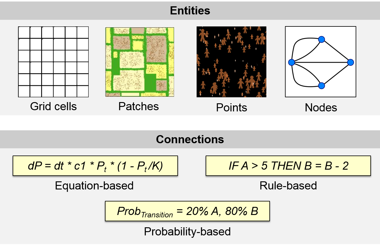
From connecting alternative representations of spatial entities with alternative representations of processes to link these entities we can derive a systematic overview of methodological approaches to spatial simulation (Figure 3.2).
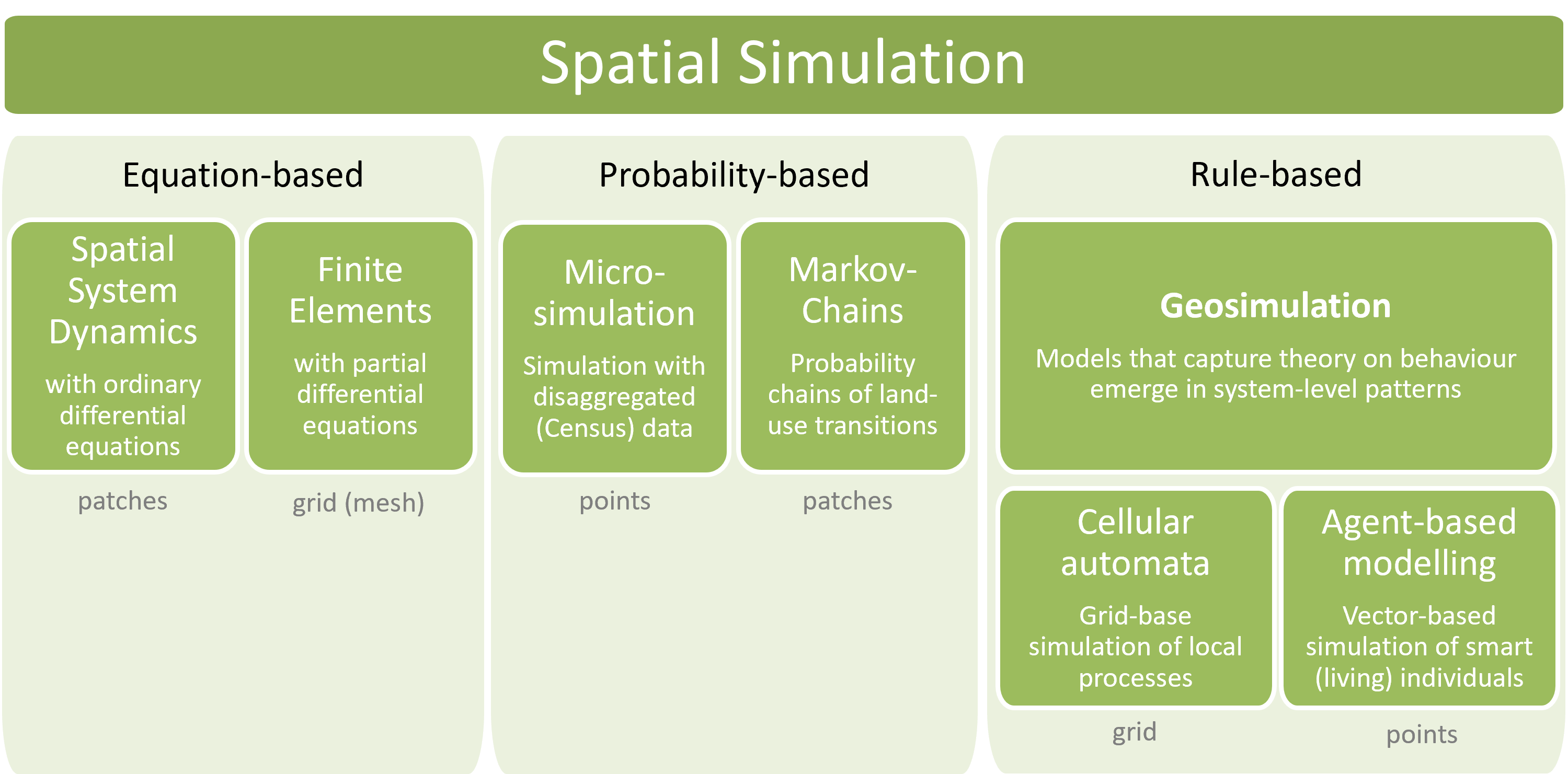
Five questions about your problem narrow the choice quickly:
| ask this about your problem | if yes, look at |
|---|---|
| Can the entities be averaged into homogeneous stocks? | Spatial System Dynamics |
| Is it a physical process that is continuous in space and time? | Partial Differential Equations |
| Do you need prediction rather than explanation? | probability-based models |
| Does variation between individuals drive the outcome? | Geosimulation |
| Must the system change its own structure - self-organise? | Geosimulation only |
The sections that follow take each in turn, and each one closes by saying when to choose that approach and when not to.
3.2 Aggregate entities: Spatial System Dynamics
A straight-forward and simple way to ‘spatialise’ a traditional System Dynamics Model is to assign a specific stock to a specific spatial entity, e.g. to a patch in a vector model or to a cell in a raster model. The forest in a patch is still modelled as an aggregate stock of e.g. biomass. This limits the level of potential spatial disaggregation: patch sizes need to hold forests that are large enough to average out individual randomness of single trees. Stocks are individual instances in the same model with the same parameterisation. Interrelations in the form of in- and out-flows and feedback loops operate independently on each stock. There are no flows between the stocks of neighbouring patches. In short, it is a model of local processes (Neuwirth et al., 2015).
In Figure 3.3, the system dynamics model governs the forest growth process of several stocks. The input of a model draws from current states of stocks in the respective patches. The actual state of the forest stock at a certain point in time therefore differs from patch to patch. System dynamics software packages can handle simple evolution models without problems.

Further levels of spatial complexity in a Spatial System Dynamics model consider:
Local parameters Each stock has its individual parameterisation of flows and feedback loops that reflect local conditions. These are still models of local processes, but these processes depend on the local environment, e.g. nutrients, solar radiation, precipitation, etc. In system dynamics software, such local dynamics can be implemented by stock-specific parameterisation of model clones.
Interaction between neighbouring patches To account for the underlying spatial structure of the system flows and feedback loops between stocks of spatially related patches are added. For example, water only flows to downhill patches and seed dispersal only happens between adjacent patches. The system dynamics software thereby needs to be aware of topological relationships between patches. The representation of such spatial relationships is not foreseen in standard System Dynamic software packages.
Multiple stocks per patch that are spatially interrelated An additional degree of complexity is added, if we not only consider one stock per patch, but multiple interrelated stocks per patch, e.g. tree biomass, water, and CO2, number of cattle. In this case we can consider one patch as an individual submodel that is connected with other submodels through their spatial arrangement. We can have different submodels of fundamentally different types, such as forests, agricultural fields and settlements. From a computational perspective, stocks are not anymore individual instances of the same model, but we now have to deal with a multi-model system, where the relation between submodels is governed by their spatial arrangement. Such systems cannot be represented by System Dynamics software alone. Its implementation usually relies on coupling with a GISystem.
Adaptive change of model structure To represent structural changes in complex systems, a model needs to have the capability of self-organisation. In such models, new features emerge, evolve and disappear: a forest may shrink in size or entirely change into a settlement area; an abandoned pasture may turn into a forest; and a road network emerges from the mobility affordances between settlements. Such emergence and self-organisation are fundamental properties of systems. However, capabilities of Spatial System Dynamics models in this regard are rare and related research in its infancy (Neuwirth et al., 2015). The limitation of system dynamics models to become truly spatial models lies in the modelling approach itself: System Dynamics models represent the world in a top-down manner: system flows are modelled at system level. Although the system can be disaggregated to a certain degree, the smallest entity still needs to represent an aggregated, homogeneous entity that reacts to flows and feedback loops.
…the entities can be averaged. Patches must be large enough that individual randomness cancels out - a forest stand, not a single tree. Choose something else if the outcome depends on entities differing from one another, or if the system has to reorganise itself: a system dynamics model cannot produce structure it was not given.
3.3 Continuous space and time: Partial Differential Equations
In order to model physical processes that are continuous in space and time, it is not enough to model a variable over time, but we need to explicitly include also space as a variable. Typical application examples that interface with geoinformatics would be fluid dynamics, like water turbulence in a river (Figure 3.5), or wind speeds around obstacles (Figure 3.4). Solid models are less relevant for geoinformatics applications. They are mainly used to simulate the behaviour of materials, e.g. deformations of cars in crash simulations.
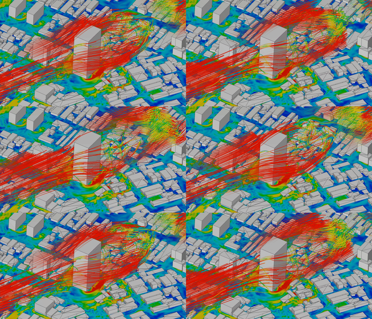
Mathematically, we have to move from ordinary differential equations that model a process over time (the system dynamics approach) to partial differential equations (PDE) that model a process in time and space. To solve partial differential equations, we do not just have to dissect time into small time steps, but also dissect space into a mesh (Figure 3.5) - and then again use numerical simulation to approximate the solution in stepwise difference equations from time step to time step and from mesh patch to mesh patch.
As you will guess, the resolution and the structure of the mesh is of great importance for the quality of the model. Areas of steep gradients afford a fine mesh, whereas more homogeneous areas can be wide-meshed to reduce computational costs.
According to the type of mesh geometry, we can distinguish Finite Difference methods based on rectangular grids, Finite Element methods based on TINs and Finite Volume methods which usually are based on voxels or Voronoi regions. The spatio-temporal patterns that result from numerical models include stationary and dynamic patchy patterns, oscillations, propagation fronts or spiral waves.
…the process is physical and continuous in both space and time, and the governing equations are known - fluid flow, heat, dispersion. Choose something else if the entities are discrete individuals, or if you cannot write down the equation that governs the process.
3.4 Correlation without mechanism: probability-based models
Probability-based spatio-temporal models rely on observation data, from which statistical relationships between spatial entities can be inferred. Probabilistic models are purely phenomenological. That means they describe the system without providing any insights into causalities and how a system functions. However, probabilistic models mimic real-world processes often very closely, which makes them perfect candidates for predictive models, like weather forecasts or the prediction of traffic congestions. The only caution that needs to be taken is that these models are only valid within the spatial and temporal frame for which they have been calibrated. Therefore, a probabilistic traffic model for instance cannot predict traffic flows around a new construction site. However, as data nowadays gets more and more abundant, probabilistic models of dynamic system gain momentum. Most prominently, this involves Markov Chain models.
A set of different machine-learning approaches would also fall under the category of correlative, probability-based models. However, the actual mechanism of the process is hidden in these models. The purpose of such “black box” models thus is shifted from understanding systems to predicting systems. A comprehensive discussion of spatio-temporal machine learning approaches would be worth another module.
3.4.1 Markov Chains
Markov Chains are an probabilistic approach for patch-based models. They define the status of a cell in the next time step, based on its own current status and a transition-probability matrix that is derived from (big)data. This matrix is sketched graphically in the diagram in Figure 3.6. For example, in a land-use change model, there might be a 10% probability for a cell with agricultural land use to change its state to urban. The probabilities can either be empirical data gathered from observations of past changes or they can be expert-based. Such ‘memoryless’ transitions, where the next state only depends on the current state are called Markov Chains.
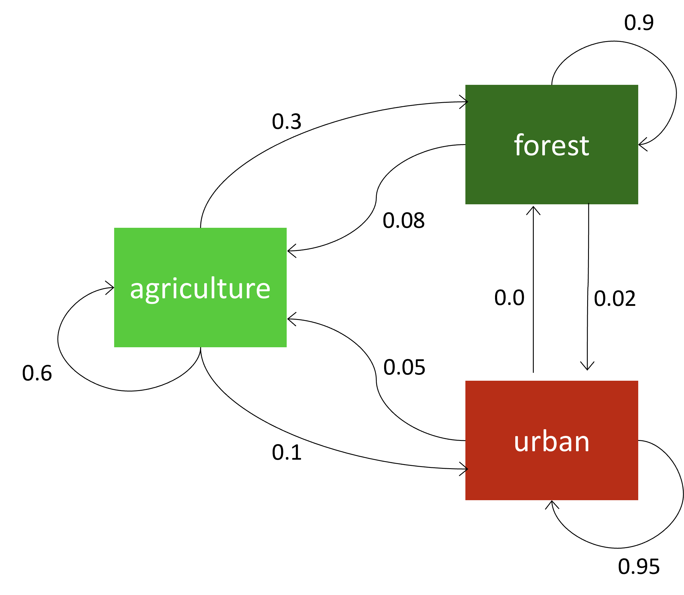
The interactive NetLogo model in Figure 3.7 implements the Markov chain transition rules of Figure 3.6. As you run the simulation, you will note that the transition between land use classes is random in space.
…you have observation data and you need prediction rather than explanation. These models mimic real processes closely without revealing why. Choose something else if you need the mechanism, or if the model will be applied outside the spatial and temporal frame it was calibrated for - a probabilistic traffic model cannot anticipate a new construction site.
3.5 Interacting individuals: Geosimulation
Geosimulation models are bottom-up models, which assume that internal heterogeneity plays an important role for the system’s structure and function. The entities are disaggregated to the level of individuals and very local environments that adapt to each other and interact locally. Thus, Geosimulation is the methodological approach to address questions around complex, living systems. The models that were presented in Chapter 2 to exemplify properties of complex systems are all geosimulation models: flocking, peppered moths, or the virus model.
In the 1970ies Simon Levin introduced the importance of spatial heterogeneity to the ecological community (Levin, 1976). Subsequently, modellers demonstrated for many processes that spatial heterogeneity can explain observed behaviour of spatial systems much better than aggregate equation-based models could, e.g. predator-prey stability (Hastings, 1977), species diversity (Rosenzweig, 1995), or the spread of wildfires in patchy landscapes (Turner & Romme, 1994).
Spatial heterogeneity is at the centre of interest in Geosimulation. Modellers have approached it from two sides: processes in heterogenous landscapes (Cellular Automata models) and heterogeneous individuals that interact locally (Agent-based models). Most often Geosimulation models are hybrid models, where individual agents of an Agent-based model interact with the local environment that is modelled as Cellular Automaton.
With Geosimulation models, we can study, how spatial patterns affect the behaviour of individuals (e.g. route choice), or vice-versa how spatial patterns emerge from the interaction of individuals (e.g. traffic jams).
…spatial heterogeneity is the point: the outcome arises because entities differ from one another and interact locally. It is the only approach here that can produce structure the modeller never specified. Choose something else if the entities really can be averaged - geosimulation then costs you complexity and computing time for nothing.
Simulation models can conceptualise a system from the top down or from the bottom up. This module focuses on the bottom-up approaches, because they disaggregate to the level of individual entities and are therefore the more relevant ones for spatial problems. Having seen what each approach can and cannot do, that focus should now read as a conclusion rather than an assumption - and the next lesson puts it into practice.
Each of the four problems below is decided by one of the five questions of Table 3.1. Match them: select a question, then select the problem it settles. One question is left over - work out which, and why.