Lesson 8 Read and Write Data
In previous exercises we have read data from a CSV file into our script. Similarly we can also write code outputs to file.
In this lesson you will learn to read and write plain-text, spatial vector and raster file formats. Moreover, we will retrieve online data by means of a data API.
8.1 Read and write tabular data
A series of formats are based on plain-text files.
For instance…
- comma-separated values files
.csv - semi-colon-separated values files
.csv - tab-separated values files
.tsv - other formats using custom delimiters
- fix-width files
.fwf
The readr library (also part of Tidyverse) provides a series of functions that can be used to load from and save to such data formats. For instance, the read_csv function reads a comma-delimited CSV file from the path provided as the first argument.
The code example below reads a CSV file that contains global fishery statistics provided by the World Bank and queries Norwegian entries. The function write_csv writes these entries to a new CSV file.
library(tidyverse)

fishery_data <- readr::read_csv("data/capture-fisheries-vs-aquaculture.csv")
# print(fishery_data)

# print(typeof(fishery_data$))

fishery_data %>%
  dplyr::filter(Entity == "Norway") %>%
  readr::write_csv("data/capture-fisheries-vs-aquaculture-norway.csv", append=FALSE) %>%

  dplyr::slice_head(n = 3) %>%
knitr::kable()| Entity | Code | Year | Aquaculture production (metric tons) | Capture fisheries production (metric tons) |
|---|---|---|---|---|
| Norway | NOR | 1960 | 1900 | 1609362 |
| Norway | NOR | 1961 | 900 | 1758413 |
| Norway | NOR | 1962 | 200 | 1572913 |
In order to run the script, download the CSV file. Then copy and run the code in a new R-script.
8.2 Read and write vector data
The library sf makes it easy to read and write vector datasets such as shapefiles.
sf library to build vector geometries from scratch. Investigate their properties and assign and transform coordinate reference systems. The name sf stands for simple features, meaning that sf-objects conform to the simple feature standard. Now we use the same library to load sf-objects from file.
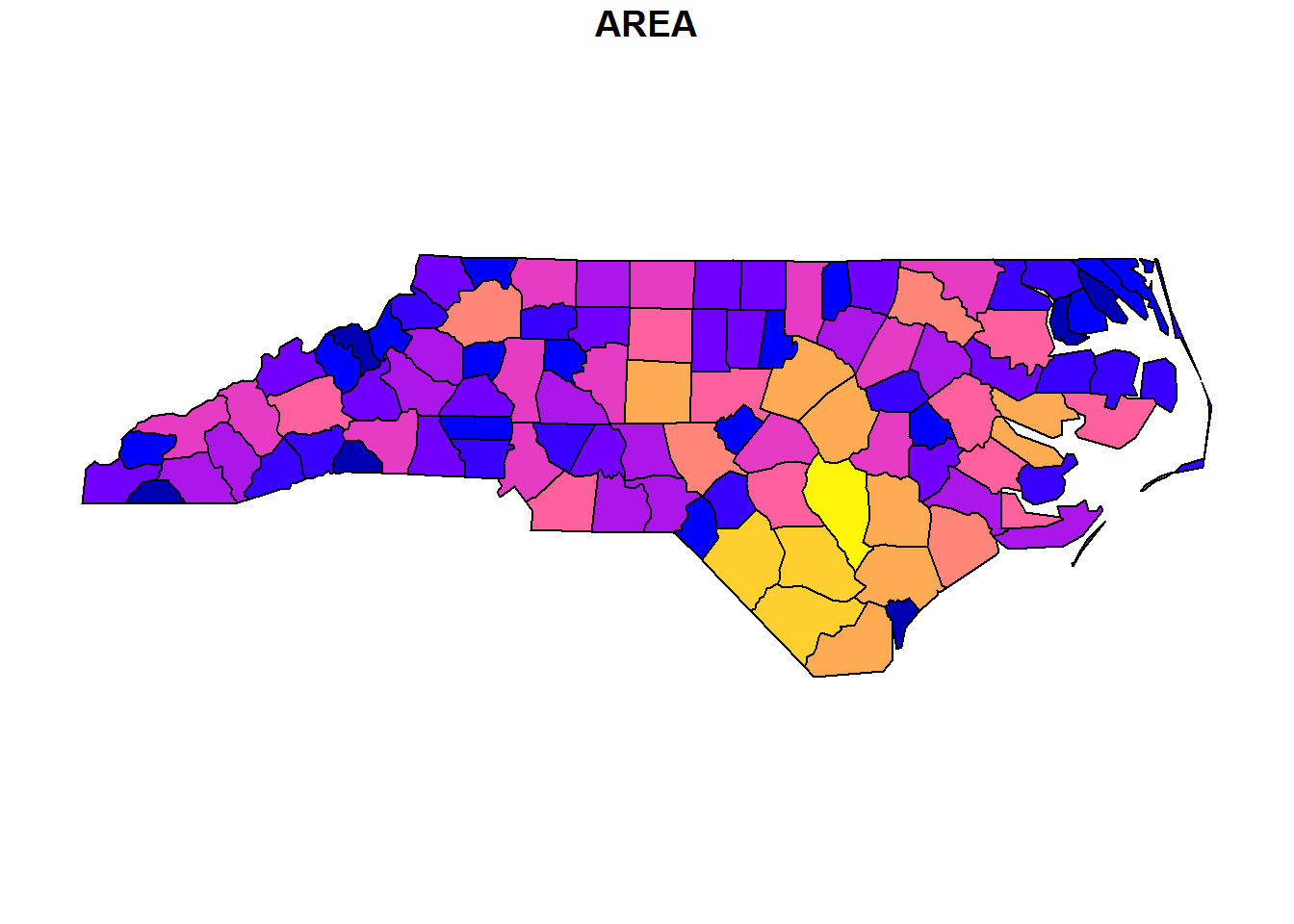
In order to load vector data in an R-Script, we can use the function st_read(). In the code block below, a shapefile (North Carolina sample data) is loaded and assigned to a variable nc.
The next line creates a basic map in sf by means of plot(). By default this creates a multi-panel plot, one sub-plot for each variable (attribute) of the sf-object.

As you have learned in lesson 4, sf represents features as records in data-frame-like structures with an additional geometry list-column. The example below renders three features (rows) of variable nc including the geometry column of type MULTIPOLYGON (see Simple feature geometry types) as well as the attributes AREA (feature area) and NAME (name of county):
| AREA | NAME | geometry |
|---|---|---|
| 0.114 | Ashe | MULTIPOLYGON (((-81.47276 3… |
| 0.061 | Alleghany | MULTIPOLYGON (((-81.23989 3… |
| 0.143 | Surry | MULTIPOLYGON (((-80.45634 3… |
sf also includes a number of operations to manipulate the geometry of features such as st_simplify:
You may have recognized that a dot (.) is used as a parameter in the function plot(). The dot represents the piped value. In the example above the dot is used to define the simplified geometry of nc as first parameter of function plot() and max.plot = 1 as the second.
In the next example, the st_geometry() retrieves the geometry attribute from variable nc, function st_centroid() calculates the centroid of the polygon geometry (counties) and function st_write writes the centroid point geometry to file.
sf::st_geometry(nc) %>%
  sf::st_centroid() %>%
  sf::st_write("data/nc-centroids.shp", delete_dsn = TRUE) %>%
plot(pch = 3, col = 'red') 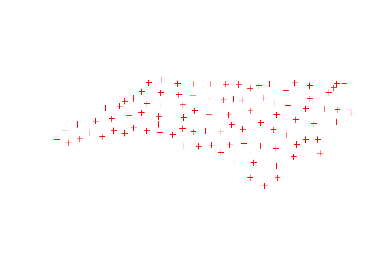
In order to test the code on your machine, download the North Carolina dataset and install the libraries sf and Rcpp before you run the code in an R-Script.
The plot() function offers a large number of arguments that can be used to customize your map. Replace ‘AREA’ in the map above by a more meaningful map title. Turn to the documentation for more information.
See our solution!
8.3 Read and write raster data
The terra library provides functions to read and write raster data. In lesson 4, we used the terra library to build SpatRaster Objects from scratch, investigated their properties and assigned and transformed coordinate reference systems.
It is more common, however, to create a SpatRaster Object from a file. Supported file formats for reading are GeoTIFF, ESRI, ENVI, and ERDAS. Most formats supported for reading can also be written to (see Creating SpatRaster objects).
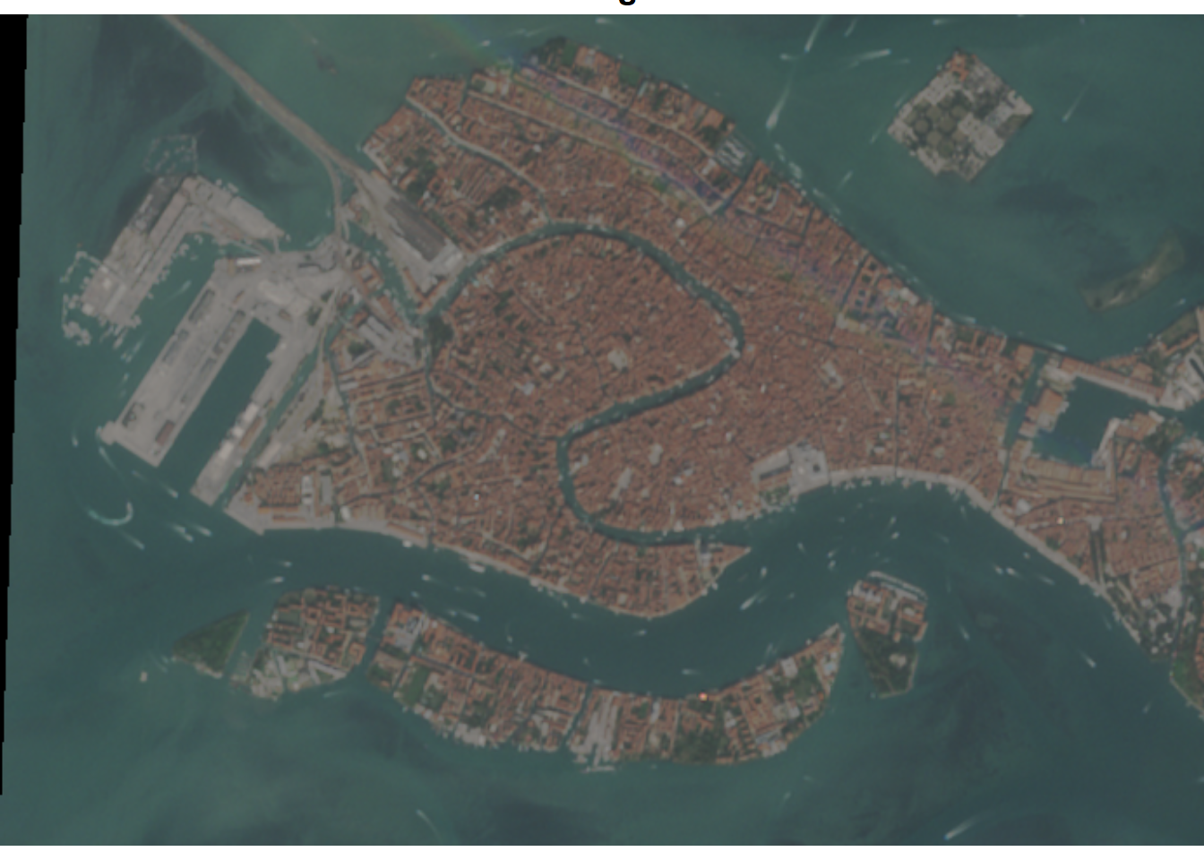
The following code reads a GeoTIFF (download venice-Sentinel.tiff 712KB) into memory and assigns it to a variable named r:
The function hasValues returns the logic value TRUE, which indicates that in-memory layers have cell values:
## [1] TRUEExecuting the variable name r returns additional metadata information, which among others reveals that the image has 4 layers:
## class       : SpatRaster
## dimensions  : 503, 692, 4  (nrow, ncol, nlyr)
## resolution  : 7.025638, 6.675899  (x, y)
## extent      : 288674.2, 293535.9, 5033073, 5036431  (xmin, xmax, ymin, ymax)
## coord. ref. : WGS 84 / UTM zone 33N (EPSG:32633)
## source      : venice-Sentinel.tiff
## names       : venice-Sentinel_1, venice-Sentinel_2, venice-Sentinel_3, venice-Sentinel_4
Layers 1-3 correspond to color bands red, green, and blue. In order to plot the true color sentinel imagery, we can use terra function plotRGB and assign the numbers of respective color bands to attributes r (red), g (greeb), b (blue):
The following line converts the original CRS (which is WGS 84 / UTM zone 33N) to the Italian national CRS Italy Zone 1:
r_z1 <- terra::project(r, "+proj=tmerc +lat_0=0 +lon_0=9 +k=0.9996 +x_0=1500000 +y_0=0 +ellps=intl +units=m +no_defs")Eventually, the modified SpatRaster Object is written to file by means of terra function writeRaster:
8.4 Data API
API is the acronym for Application Programming Interface, which is a software intermediary that allows two applications to talk to each other.
By means of an API we can read, write, and modify information on the web. The following video briefly introduces the technology behind it.
Figure 8.1: Video (3:13 min): REST API concepts and examples.
The most important takeaway messages are:
- With a REST API, web data is accessible through a URL (Client-Server call via HTTP protocol)
- The HTTP Get Method delivers data (a Response) - i.e. is used to read data, the HTTP Post Method is used to create new REST API resources (write data).
- URL Parameters are used to filter specific data from a response.
- Typically, APIs can return data in a number of different formats.
- JSON is a very popular format for transferring web data.
- The two primary elements that make up JSON are keys and values.
The library httr2 offers functions to programmatically implement API calls in an R script. We will make use of this library to let our R script interact with the APIs offered by Geosphere Austria that contains historical weather data and weather forecasts in time series or gridded formats for retrieval. In the upcoming example we will make a call to the INCA Dataset, which offers hourly data on temperature, precipitation, wind, solar radiation, humidity and air pressure.
For accessing the data with httr2, we’ll construct a URL composed of a reference to the data source (base), and parameters to filter the desired data subset. To assemble base URL and parameters we will use the function sprintf().
sprintf() function in R is used for string formatting. It allows you to combine, format, and interpolate variables into strings in a flexible way. For example, sprintf("%s?parameters=%s&start=%s", base, lat, lon) constructs a URL string by inserting the values of base, lat and lon into the placeholders (%s). Each %s is replaced by the corresponding variable’s value in the order they are listed. This function is particularly useful in scenarios where you need to dynamically generate strings or URLs with variable data.
library(httr2)

# Define the base URL and parameters
base <- "https://dataset.api.hub.geosphere.at/v1/timeseries/historical/inca-v1-1h-1km"
parameters <- "T2M"
start_date <- "2023-06-01T22:00"
end_date <- "2023-06-01T22:00"
latlon <- "47.81,13.03"
output_format <- "geojson"

# Construct the full URL with query parameters using sprintf
full_url <- sprintf("%s?parameters=%s&start=%s&end=%s&lat_lon=%s&output_format=%s", base, parameters, start_date, end_date, latlon, output_format)

# Display the constructed URL
print(full_url)
## [1] "https://dataset.api.hub.geosphere.at/v1/timeseries/historical/inca-v1-1h-1km?parameters=T2M&start=2023-06-01T22:00&end=2023-06-01T22:00&lat_lon=47.81,13.03&output_format=geojson"The base URL (base) in the code above specifies version (v1), type (timeseries), mode (historical) and resource-id (inca-v1-1h-1km) of the dataset being requested. This structure is described under Endpoint Structure in the API Documentation.
All datasets as well as available types, modes and response formats can be listed via https://dataset.api.hub.geosphere.at/v1/datasets.
Additional metadata of the endpoint can be requested by appending /metadata to the base URL. For instance, https://dataset.api.hub.geosphere.at/v1/timeseries/historical/inca-v1-1h-1km/metadata returns a JSON that lists information on the resolution (hourly), temporal and spatial extent of the data as well as variables (parameters) and formats (output_format) that are available with this endpoint.
Before you assemble request URLs, it is recommended to test different calibrations in the FastAPI frontend.
The assembled request URL full_url (see code above) retrieves air temperature 2m above ground (T2M) for an individual point in time (2023-06-01T22:00) as geojson from the INCA dataset, which is a time series with hourly resolution.
As a next step, the URL is passed to the request() function to create a request object, and req_perform() is used to execute the HTTP Get method:
By default, the req_perform() function returns a response object. Printing a response object provides useful information such as the actual URL used (after any redirects), the HTTP status, and the content type.
You can extract important parts of the response with various helper functions such as resp_status() and resp_body_json():
## [1] 200## List of 5
## $ media_type: chr "application/json"
## $ type : chr "FeatureCollection"
## $ version : chr "v1"
## $ timestamps:List of 1
## ..$ : chr "2023-06-01T22:00+00:00"
## $ features :List of 1
## ..$ :List of 3
## .. ..$ type : chr "Feature"
## .. ..$ geometry :List of 2
## .. .. ..$ type : chr "Point"
## .. .. ..$ coordinates:List of 2
## .. .. .. ..$ : num 13
## .. .. .. ..$ : num 47.8
## .. ..$ properties:List of 1
## .. .. ..$ parameters:List of 1
## .. .. .. ..$ T2M:List of 3
## .. .. .. .. ..$ name: chr "air temperature"
## .. .. .. .. ..$ unit: chr "degree_Celsius"
## .. .. .. .. ..$ data:List of 1
## .. .. .. .. .. ..$ : num 16.3To facilitate subsequent analyses and data visualization, we can convert the content of the return object to a data frame. With httr2, you can directly retrieve the JSON content and convert it to a data frame:
library(knitr)

# Using resp_body_json to get the JSON content of the response
response_content <- httr2::resp_body_json(resp)
response_df <- as.data.frame(response_content)

# Select columns 7, 8, 10 and 11 of response data frame
# rename columns and render data frame as html table
names <- c("X", "Y", "unit", "temp")
response_df %>%
  dplyr::select(7, 8, 10, 11) %>%
  setNames(., names) %>%
knitr::kable(., format="html")| X | Y | unit | temp |
|---|---|---|---|
| 13.02537 | 47.81396 | degree_Celsius | 16.29 |
For purposes of presentation, the returned data frame was shortened to show only four columns.