Lesson 7 Data Manipulation
In most instances, the structure of the available data will not meet the specific requirements needed to perform the analyses you are interested in. Data analysts typically spend most of their time cleaning, filtering, restructuring data as well as harmonizing and joining data from different sources.
In this lesson, you will learn about the fundamental data wrangling operations using the dplyr library from the Tidyverse suite. You’ll also be introduced to tibbles, a modern take on data frames in R. Tibbles are lightweight and work seamlessly within the Tidyverse ecosystem. For more on tibbles, see Tibbles in R for Data Science.
7.1 Preparation
If not already installed on your machine, install both the tidyverse and nycflights13 libraries. (see “libraries” in lesson 2).
The code below loads a sample dataset (a tibble) from the library nycflights13 into the variable flights_from_nyc. We will use this sample data in this lesson.
The operator :: is used to indicate that the function flights (that returns our sample dataset) is situated within the library nycflights13. This helps avoid ambiguities when functions from different loaded libraries have the same names.
In order to run the following data wrangling examples on your machine, add both lines above as well as the code snippets provided in the upcoming examples to a new R script file.
Once you have loaded the flights table, open the Environment Tab in RStudio and double-click variable flights_from_nyc to inspect the variable contents.
Alternatively, you may inspect flights_from_nyc by writing it to the console.
7.2 Data manipulation
The dplyr library provides a number of functions to investigate the basic characteristics of inputs. For instance, the function count() can be used to count the number of rows of a data frame or tibble. The code below uses flights_from_nyc as input to this function. The returned row count n is represented in a table.
| n |
|---|
| 336776 |
In the example above, we use the pipe operator %>%, a key feature of magrittr and tidyverse syntax. The operator links a sequence of analysis steps, passing flights_from_nyc through count() and then kable(). This makes the code simpler and more readable. For a deeper understanding, check out this video.
The same result could be achieved with a traditional approach using an intermediate variable or by nesting functions. However, these methods can make the code less readable compared to using the pipe operator:
Intermediate Variable:
Nested Function:
The result is the same. However, nested structures are harder to read. Accordingly, the pipe operator is a powerful tool to simplify your code. See this video to learn more about it.
The function count() can also be used to count the number of rows of a table that has the same value for a given column, usually representing a category.
In the example below, the column name origin is provided as an argument to the function count(), so rows representing flights from the same origin are counted together – EWR is the Newark Liberty International Airport, JFK is the John F. Kennedy International Airport, and LGA is LaGuardia Airport.
| origin | n |
|---|---|
| EWR | 120835 |
| JFK | 111279 |
| LGA | 104662 |
Notice how the code becomes more readable with each operation on a new line after %>%. Remember, the pipe operator passes the left-hand object as the first argument to the right-hand function. To change the argument placement, use . within the function call.
For example, you could explicitly pass variable flights_from_nyc as a first argument by dplyr::count(., origin). Passing the variable as a second argument dplyr::count(origin, .) will return an error as the data frame is expected as a first input to function count.
7.2.1 Summarise
To carry out more complex aggregations, the function summarise() can be used in combination with the function group_by() to summarise the values of the rows of a data frame or tibble. Rows having the same value for a selected column (in the example below, the same origin) are grouped together, then values are aggregated based on the defined function (using one or more columns in the calculation).
In the example below, the function mean() is applied to the column distance to calculate a new column mean_distance_traveled_from (the mean distance travelled by flights starting from each airport).
flights_from_nyc %>%
  dplyr::group_by(origin) %>%
  dplyr::summarise(
    mean_distance_traveled_from = mean(distance)
  ) %>%
knitr::kable()| origin | mean_distance_traveled_from |
|---|---|
| EWR | 1056.7428 |
| JFK | 1266.2491 |
| LGA | 779.8357 |
The results show that the average distance covered by flights starting from JFK is significantly higher that flights departing from LGA or EWR.
7.2.2 Select and filter
The function select() can be used to select a subset of columns. For instance in the code below, the function select() is used to select the columns origin, dest, and dep_delay. The function slice_head is used to include only the first n rows in the output.
flights_from_nyc %>%
  dplyr::select(origin, dest, dep_delay) %>%
  dplyr::slice_head(n = 5) %>%
knitr::kable()| origin | dest | dep_delay |
|---|---|---|
| EWR | IAH | 2 |
| LGA | IAH | 4 |
| JFK | MIA | 2 |
| JFK | BQN | -1 |
| LGA | ATL | -6 |
The function filter() can instead be used to filter rows based on a specified condition. In the example below, the output of the filter step only includes the rows where the value of month is 11 (i.e., the eleventh month, November).
flights_from_nyc %>%
  dplyr::select(origin, dest, year, month, day, dep_delay) %>%
  dplyr::filter(month == 11) %>%
  dplyr::slice_head(n = 5) %>%
knitr::kable()| origin | dest | year | month | day | dep_delay |
|---|---|---|---|---|---|
| JFK | PSE | 2013 | 11 | 1 | 6 |
| JFK | SYR | 2013 | 11 | 1 | 105 |
| EWR | CLT | 2013 | 11 | 1 | -5 |
| LGA | IAH | 2013 | 11 | 1 | -6 |
| JFK | MIA | 2013 | 11 | 1 | -3 |
Notice how filter is used in combination with select. All functions in the dplyr library can be combined, in any other order that makes logical sense. However, if the select step didn’t include month, that same column couldn’t have been used in the filter step.
7.2.3 Mutate
The function mutate() can be used to add a new column to an output table. The mutate step in the code below adds a new column air_time_hours to the table obtained through the pipe, that is the flight air time in hours, dividing the flight air time in minutes by 60.
flights_from_nyc %>%
  dplyr::select(flight, origin, dest, air_time) %>%
  dplyr::mutate(
    air_time_hours = air_time / 60
  ) %>%
  dplyr::slice_head(n = 5) %>%
knitr::kable()| flight | origin | dest | air_time | air_time_hours |
|---|---|---|---|---|
| 1545 | EWR | IAH | 227 | 3.783333 |
| 1714 | LGA | IAH | 227 | 3.783333 |
| 1141 | JFK | MIA | 160 | 2.666667 |
| 725 | JFK | BQN | 183 | 3.050000 |
| 461 | LGA | ATL | 116 | 1.933333 |
Run the mutate example above in a new script and replace dplyr::mutate with dplyr::transmute. What happens to your results?
See solution!
The transmute function creates a new data frame containing only column air_time_hours. The function drops other table columns.
7.2.4 Arrange
The function arrange() sorts a `tibble or data frame in ascending order based on the values in the specified column. If a negative sign is specified before the column name, the descending order is used. The code below would produce a table showing all the rows when ordered by descending order of air time.
flights_from_nyc %>%
  dplyr::select(origin, dest, air_time) %>%
  dplyr::arrange(-air_time) %>%
  dplyr::slice_head(n = 5) %>%
knitr::kable()| origin | dest | air_time |
|---|---|---|
| EWR | HNL | 695 |
| JFK | HNL | 691 |
| JFK | HNL | 686 |
| JFK | HNL | 686 |
| JFK | HNL | 683 |
In the examples above, we have used slice_head to present only the first n rows in a table, based on the existing order.
7.2.5 Exercise: data manipulation
The Food and Agriculture Organization (FAO) is a specialized agency of the United Nations that leads international efforts to defeat hunger. On their Website they provide comprehensive datasets on global crop and livestock production. Your task in this exercise is to create a table that shows national African sorghum production in 2019.
- Create an RScript and install or load the libraries
tidyverseandknitr, if not done yet. - Bulk download African Crop and Livestock Production data as CSV:
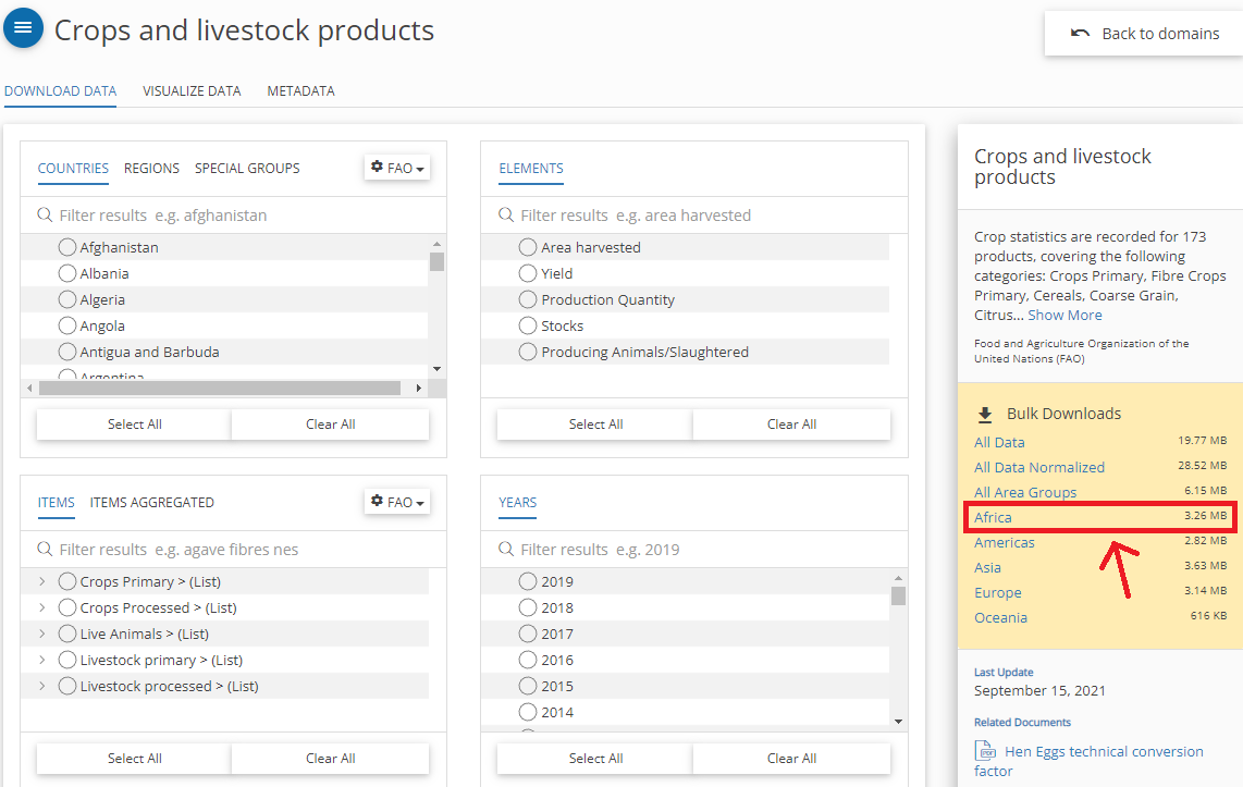
Figure 7.1: FAO Data Download
- Read data from comma-separated CSV (
"Production_Crops_Livestock_E_Africa_NOFLAG.csv") into your Script.
fao_data <- read.csv(directory as string, header = TRUE, sep = ",")- Use the pipe operator to perform the following operations:
- Select columns
Area,Item,Element,UnitandY2019 - Filter rows that contain sorghum production (
Item == "Sorghum" & Element == "Production") - Sort the table based on yield in descending order (
arrange) - remove rows including
No Databy means of functiondrop_na() - render the table using the function
kable()oflibrary knitr
- Select columns
See my solution!
Note on Encoding: When working with datasets from various sources, you may encounter encoding errors. If such an issue arises, a simple approach is to specify the encoding in the read.csv() function. For instance, you can use read.csv(..., fileEncoding = "latin1"). However, the best case would be, to check the original encoding of the data beforehand and match it in your read.csv() command. Encoding can be tricky, and while it’s outside the scope of this exercise, being aware of it is crucial in data analysis.
7.3 Join
A join operation combines two tables into one by matching rows that have the same values in a specified column. This operation is usually executed on columns containing identifiers, which are matched through different tables containing different data about the same real-world entities.
For instance, the table created below (data frame city_telephone_prexix) contains the telephone prefixes of three cities.
city_telephone_prexix <- data.frame(
    city = c("Leicester", "Birmingham", "London"),
    telephon_prefix = c("0116", "0121", "0171")
  ) %>%
  tibble::as_tibble()

city_telephone_prexix %>%
knitr::kable()| city | telephon_prefix |
|---|---|
| Leicester | 0116 |
| Birmingham | 0121 |
| London | 0171 |
That information can be combined with the data present in a second table city_info_wide (see below) through the join operation on the columns containing the city names.
city_info_wide <- data.frame(
    city = c("Leicester", "Nottingham"),
    population = c(329839, 321500),
    area = c(73.3, 74.6),
    density = c(4500, 4412)
  ) %>%
  tibble::as_tibble()

city_info_wide %>%
knitr::kable()| city | population | area | density |
|---|---|---|---|
| Leicester | 329839 | 73.3 | 4500 |
| Nottingham | 321500 | 74.6 | 4412 |
kable() function requires tibbles as input.
Joins between two tables can be executed by different join operations. The dplyr library offers join operations, which correspond to SQL joins illustrated in the image below.
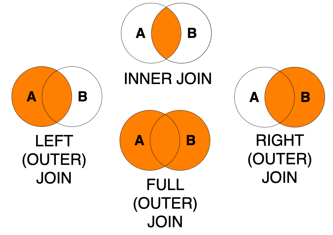
Figure 7.2: Join types
Please take your time to understand the examples below that show different realizations of joins between table city_telephone_prexix and table city_info_wide.
The first four examples execute the exact same full join operation using three different syntaxes: with or without using the pipe operator and specifying the by argument or not. Note that all those approaches to writing the join are valid and produce the same result. The choice about which approach to use will depend on the code you are writing. In particular, you might find it useful to use the syntax that uses the pipe operator when the join operation is itself only one stem in a series of data manipulation steps. Using the by argument is usually advisable unless you are certain that you aim to join two tables with all and exactly the column that have the same names in the two table.
Note how the result of the join operations is not saved to a variable. The function knitr::kable is added after each join operation through a pipe %>% to display the resulting table in a nice format.
# Option 1: without using the pipe operator
# full join verb
dplyr::full_join(
    # left table
    city_info_wide,
    # right table
    city_telephone_prexix,
    # columns to match
    by = c("city" = "city")
  ) %>%
knitr::kable()| city | population | area | density | telephon_prefix |
|---|---|---|---|---|
| Leicester | 329839 | 73.3 | 4500 | 0116 |
| Nottingham | 321500 | 74.6 | 4412 | NA |
| Birmingham | NA | NA | NA | 0121 |
| London | NA | NA | NA | 0171 |
# Option 2: without using the pipe operator
#   and without using the argument "by"
#   as columns have the same name
#   in the two tables.
# Same result as Option 1
# full join verb
dplyr::full_join(
    # left table
    city_info_wide,
    # right table
    city_telephone_prexix
  ) %>%
knitr::kable()| city | population | area | density | telephon_prefix |
|---|---|---|---|---|
| Leicester | 329839 | 73.3 | 4500 | 0116 |
| Nottingham | 321500 | 74.6 | 4412 | NA |
| Birmingham | NA | NA | NA | 0121 |
| London | NA | NA | NA | 0171 |
# Option 3: using the pipe operator
#   and without using the argument "by"
#   as columns have the same name
#   in the two tables.
# Same result as Option 1 and 2
# left table
city_info_wide %>%
  # full join verb
  dplyr::full_join(
    # right table
    city_telephone_prexix
  ) %>%
knitr::kable()| city | population | area | density | telephon_prefix |
|---|---|---|---|---|
| Leicester | 329839 | 73.3 | 4500 | 0116 |
| Nottingham | 321500 | 74.6 | 4412 | NA |
| Birmingham | NA | NA | NA | 0121 |
| London | NA | NA | NA | 0171 |
# Option 4: using the pipe operator
#   and using the argument "by".
# Same result as Option 1, 2 and 3
# left table
city_info_wide %>%
  # full join verb
  dplyr::full_join(
    # right table
    city_telephone_prexix,
    # columns to match
    by = c("city" = "city")
  ) %>%
knitr::kable()| city | population | area | density | telephon_prefix |
|---|---|---|---|---|
| Leicester | 329839 | 73.3 | 4500 | 0116 |
| Nottingham | 321500 | 74.6 | 4412 | NA |
| Birmingham | NA | NA | NA | 0121 |
| London | NA | NA | NA | 0171 |
# Left join
# Using syntax similar to Option 1 above
# left join
dplyr::left_join(
    # left table
    city_info_wide,
    # right table
    city_telephone_prexix,
    # columns to match
    by = c("city" = "city")
  ) %>%
knitr::kable()| city | population | area | density | telephon_prefix |
|---|---|---|---|---|
| Leicester | 329839 | 73.3 | 4500 | 0116 |
| Nottingham | 321500 | 74.6 | 4412 | NA |
# Right join
# Using syntax similar to Option 2 above
# right join verb
dplyr::right_join(
    # left table
    city_info_wide,
    # right table
    city_telephone_prexix
  ) %>%
knitr::kable()| city | population | area | density | telephon_prefix |
|---|---|---|---|---|
| Leicester | 329839 | 73.3 | 4500 | 0116 |
| Birmingham | NA | NA | NA | 0121 |
| London | NA | NA | NA | 0171 |
# Inner join
# Using syntax similar to Option 3 above
# left table
city_info_wide %>%
  # inner join
  dplyr::inner_join(
    # right table
    city_telephone_prexix
  ) %>%
knitr::kable()| city | population | area | density | telephon_prefix |
|---|---|---|---|---|
| Leicester | 329839 | 73.3 | 4500 | 0116 |
Compare the results of respective full, left, right and inner join operations. Turn to the discussion forum in case you need further explanations.
7.3.1 Exercise: join
In the previous exercise, we created a table that shows national African sorghum production in 2019. In this exercise we will join crop production statistics with a table that contains national boundaries and visualize sorghum production quantities in a simple map.
Create an RScript and install and load the libraries
tidyverse,knitr,ggplot2andmaps, if not done yet.Copy the code from the previous exercise into your new RScript. Note that the result of the pipe operations is not saved to a variable. Save it to a variable.
Use the
ggplot2functionmap_datato convert the built in sample datasetworld(comes with librarymaps) to a data frame:
world_ctry <- map_data("world") Inspect the structure of this data frame. Every row represents a node (defined by long/lat) of a polygon feature (national boundaries).
Join tables (left table: geographic features, right table: sorghum production statistics) based on country names. Make sure to choose a join method (
full_join,inner_join,left_joinorright_join) that allows for retaining all the geographic features.
Our exercise solution creates a simple output map. Don’t worry in Lesson 10 we will cover visualization methods in more detail.
Take a look at the dplyr Cheatsheet which shows the most important dplyr operations at a glance.