Lesson 11 R Markdown

This lesson is dedicated to the rmarkdown library. However, R Markdown is more than just a library, RMarkdown is part of a set of tools designed to enhance the reproducibility of your work. Other tools and platforms such as GitHub, Jupyter, Docker, ArXiv, and bioRxiv can facilitate reproducibility in various ways. In this module, we won’t explore the paradigm of reproducible research in detail. Instead, our focus will be on how to use RMarkdown to make your analyses and reports more appealing, interactive, and efficient.

In this lesson, we will weave together code and text in professionally rendered R Markdown documents and use GitHub to safely store, share, and administer our results.

11.1 Set up your work environment

Before creating your first R Markdown document, we need to set up the GitHub environment. Originally founded as a platform for software developers, GitHub’s architecture is designed to manage changes made during software development. This architecture is also beneficial for version control of documents or any information collection.

Version control is especially important when working in teams, as it helps synchronize efforts among project participants. However, GitHub is also a reliable and open online platform for individual work, providing change tracking, documentation, and sharing features.

To set up your personal GitHub environment, follow these steps:

1. Review the Hello-World Section in GitHub’s Quickstart Documentation. Initially, reading it is sufficient—no need to complete the tutorial yet.
2. Create a GitHub account.
3. Download and install Git. Git is a distributed VCS (version control system) that mirrors the codebase and its full history on every computer. GitHub is a web-based interface that integrates seamlessly with Git. For a clear explanation of Git’s core concepts, watch this video.
4. In RStudio (under Tools > Global Options > Git / SVN), check “enable version control” and set the path to git.exe (e.g., C:/Program Files/Git/bin/git.exe). Restart RStudio afterward.
5. Create a repository on GitHub. In the tutorial, skip the section ‘Commit your first changes’.
6. By default, your repository will have one branch named main. Create an additional branch called dev off the main. Follow the instructions in the Hello-World Tutorial for guidance.

Next, install the rmarkdown library and tinytex in RStudio as described in the R Markdown Guide.

To properly installtinytex, execute both lines in RStudio:

install.packages('tinytex')
tinytex::install_tinytex()  # install TinyTeX

Follow RStudio’s prompts to install any dependencies. For technical issues, please consult the discussion forum.

11.2 Create a local clone

To work on your repository locally, you will need to create a local clone of your online GitHub repository. Here’s how:

In RStudio, go to (File > New Project > Version Control > Git).

Enter the URL of your online repository (find this URL in your GitHub repository) and select a local directory for the clone. Then click “Create Project” (refer to Fig. 11.1).

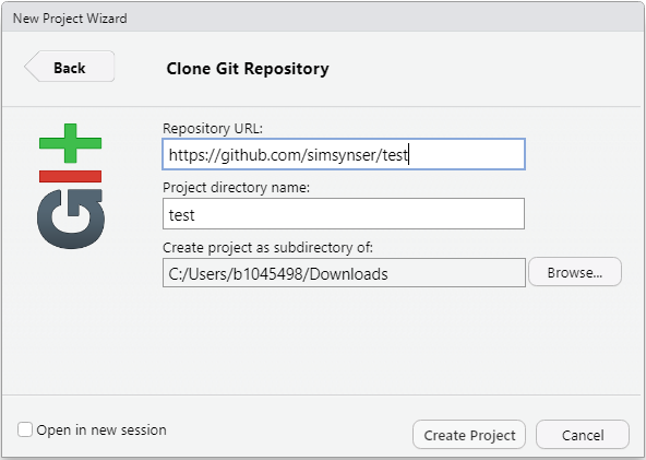
Figure 11.1: Clone GitHub Repository

Once you have cloned the online repository, the file contents of the repository as well as a new tab called “Git” appears in RStudio (see Fig. 11.2).

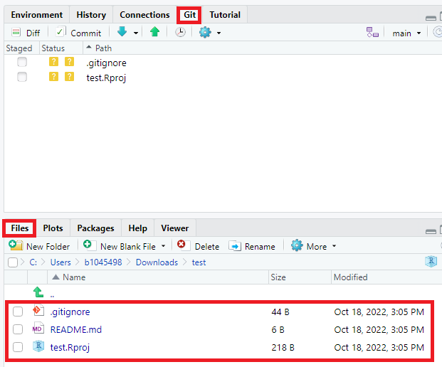
Figure 11.2: New features in RStudio

By default, the repository includes three files:

1. .gitignore: Specifies intentionally untracked files to ignore.
2. RStudio Project File (.Rproj): Contains metadata for the RStudio project.
3. ReadMe File (.md): A markdown file with information about the repository.

The gitignore and .Rproj files are created during project initialization and are not yet in the online repository. Modifications appear in the “Git” tab (Fig. 11.3).

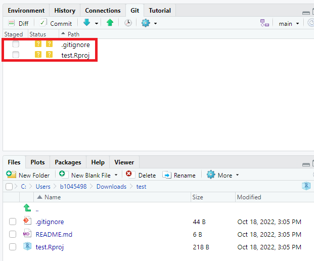
Figure 11.3: Changes in Git tab

Before making further changes, switch to the dev branch (see Fig. 11.4). At this point, the dev branch mirrors the main branch.

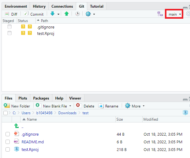
Figure 11.4: Switch branch

It is highly recommended to work in progress on a separate developer branch, like dev, and keep the main branch for stable versions. You can later merge changes from dev to main through a pull request (see Opening a Pull Request).

11.3 Creating Your First R Markdown Document

Now that the environment is set up, let’s create our first R Markdown document.

In RStudio: Navigate to (File > New File > R Markdown). Enter a title for your document, accept the default settings, and click “OK”. You’ll receive a sample R Markdown file with the extension .Rmd.

An R Markdown document comprises three core components: metadata, text and code (see Fig. 11.5).

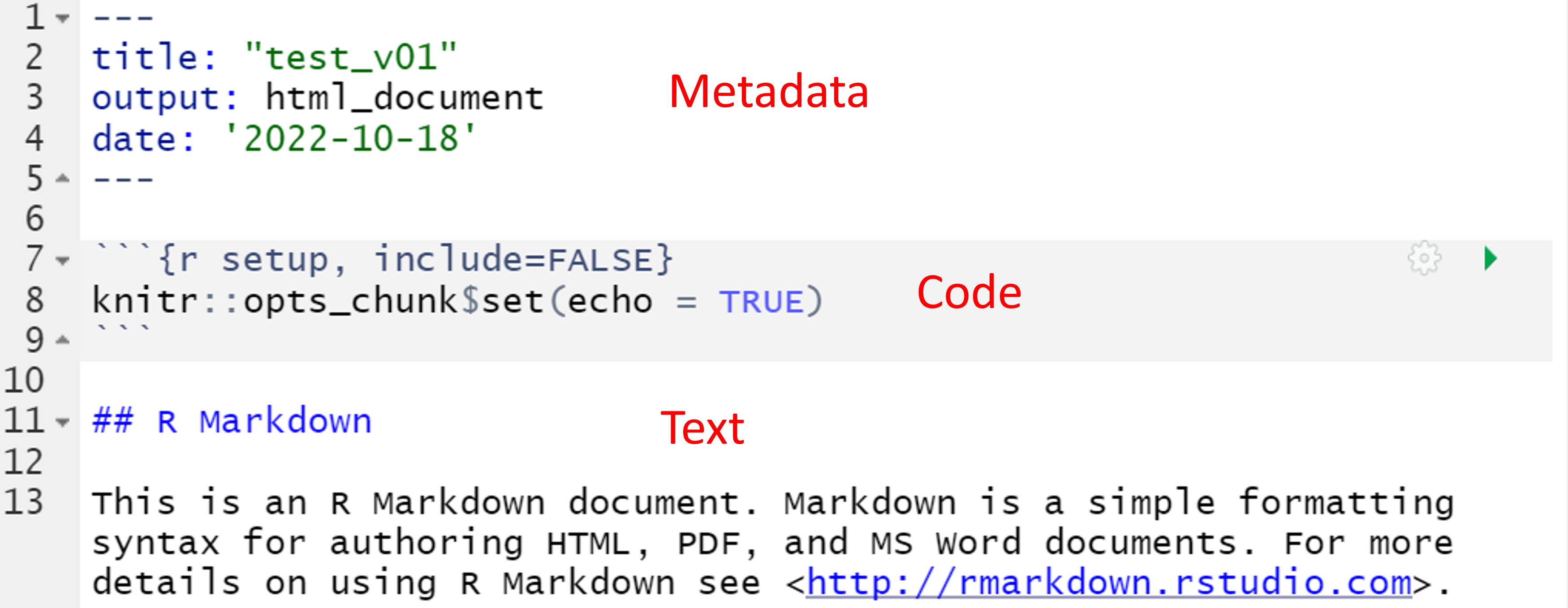
Figure 11.5: R Markdown sample file

The metadata, written in YAML syntax, defines document properties like title, output format, and creation date. Explore more about YAML syntax and document properties here.

To automatically update the date in your document, insert date: "```r format(Sys.time(), '%d %B, %Y')```" in the metadata section. This outputs the current date based on your system’s time zone in a human-readable format.

After the metadata section an R inline code block starts and ends with three backticks (see Fig. 11.5). The three parameters in curly brackets identify the code as R code. The r specifies the programming language, which is the default for R. Alternatively, you can also use parameter {py} to insert Python code into your markdown document (see Fig. 11.6).

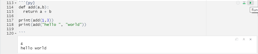
Figure 11.6: Python Example

The setup parameter specifies the name of the code block and (as we will see later) include=FALSE prevents the code and code results from being displayed in the compiled HTML output. Nevertheless, RMarkdown still runs the code in this block, which sets echo=TRUE as the default option for all code blocks in the RMarkdown document. This means that, by default, the code of all code blocks in the document will be displayed in the output file unless otherwise indicated.

Explore more about code block options in the knitr documentation.

The other code blocks in the RMarkdown sample file produce a summary output (see line 17-19) or create a simple scatterplot (see line 25-27). To see how the compiled HTML output looks like, click “Knit” (see Fig. 11.7).

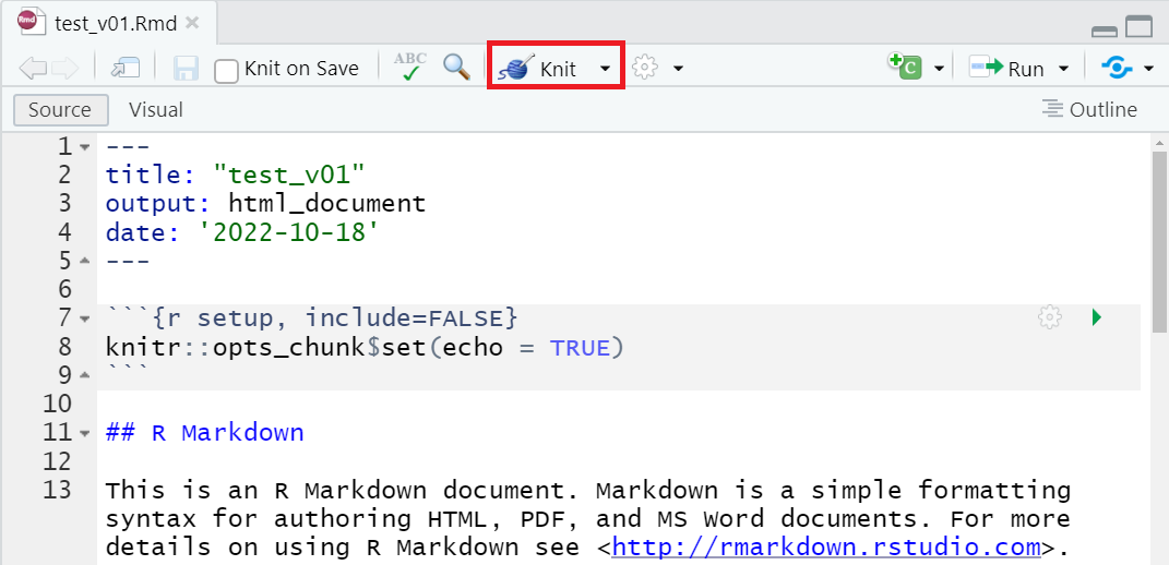
Figure 11.7: Knit HTML Output

Use the dropdown next to the “Knit” button to compile into formats such as PDF or .docx, among others.

Knitting an R Markdown document involves a two-step process. First, the .Rmd file is processed by the knitr package, which executes the code chunks and generates a new markdown file with the code and its output. Then, pandoc converts this markdown file into the final output document in the chosen format, allowing a wide range of output options for creating professional-quality documents.

11.4 Synchronizing with GitHub

Regular synchronization of your local changes with the online repository is a key practice in version control. Start by pulling any updates from the repository.

In the RStudio Git tab, click the “Pull” button (see Fig. 11.8). A notification should indicate whether any new changes are available (e.g., Already up to date).

Figure 11.8: Make Pull

Even if you’re working on your own, it’s a good idea to routinely start the sync process with a “Pull”.

Next, commit your changes. Think of committing as taking a snapshot of your progress, accompanied by a descriptive message.

First, save all documents in RStudio. Then, hit the “Commit” button in the Git tab. The commit window will display a list of modified files. Green highlights indicate new content; red highlights show deleted content.

Check the boxes next to each file to include them in the commit. Alternatively, run git add -A in the terminal to add all files at once (see this list of popular Git commands). After selecting files, enter a meaningful commit message and click “Commit”.

See Fig. 11.9.

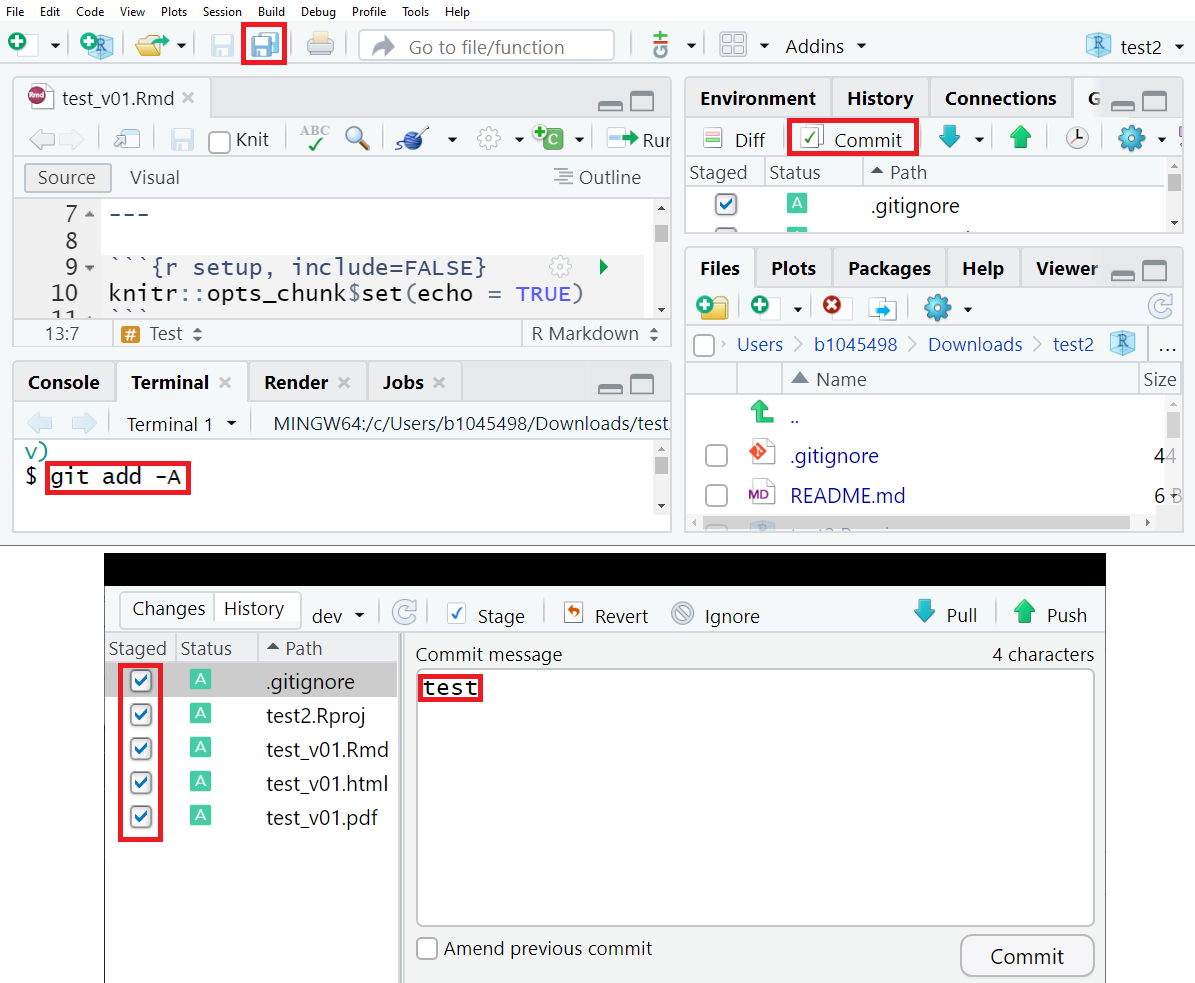
Figure 11.9: Make Commit

 

Finally, push your committed changes to the online repository.

Figure 11.10: Make Push

 

Your online repository on GitHub should now be updated (switch to dev branch in your repository) (see Fig. 11.11).

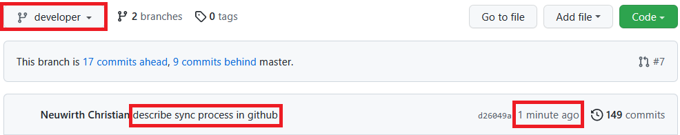
Figure 11.11: Commit with message ‘describe sync process in GitHub’ was pushed to the developer branch a minute ago

11.5 Basic R Markdown Syntax

In R Markdown, you can apply text formatting using simple markers:

Bold: Double asterisks **Text** turn text bold. Italicize: Single asterisks *Text* create italicized text. Headings: Use hash signs # for headings. The number of hashes denotes the heading level:

# Heading level 1

## Heading level 2

### Heading level 3

Tables are created by using the symbols | and -. Recall the numeric operators table from the first lesson. Figure 11.12 shows the RMarkdown syntax used for that table:

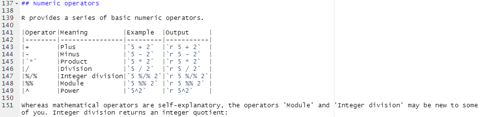
Figure 11.12: How Tables are made in Markdown

To create an ordered list, use numbers followed by a period. The first item should start with the number 1:

Code - Ordered List:
1. item 1
4. item 2
3. Item 3
    + Item 3a
    + Item 3b

Will result in:

1. Item 1
2. Item 2
3. Item 3
   • Item 3a
   • Item 3b

To create an unordered list, use *, -, or +:

Code - Unordered List:
* item 1
* item 2
  * Item 3.1
  - Item 3.2

Which will result in:

• Item 1
• Item 2
  • Item 2a
  • Item 2b

Hyperlinks are created with the format [Text](URL), for example, [GitHub](https://github.com/){target="_blank"} becomes GitHub. The target="_blank" parameter opens the link in a new tab, which is a good practice when linking to external websites.

Blockquotes are indicated by > and can be nested:

>"Everything is related to everything else, but near things are more related than distant things".
>
>>The phenomenon external to an area of interest affects what goes on inside.

Will result in:

The first law of geography is: “Everything is related to everything else, but near things are more related than distant things”

The phenomenon external to an area of interest affects what goes on inside.

Meanwhile, you know a number of characters that have a special meaning in RMarkdown syntax (like # or >). If you want these characters verbatim, you have to escape them. The way to escape a special character is to add a backslash before. For instance, # will not translate into a heading, but will return #.

RMarkdown supports a large number of mathematical notations using dollar signs $:

Math. notation example 1:

$x = y$

Result looks like:

\(x = y\)

Math. notation example 2:

$\frac{\partial f}{\partial x}$

Result looks like:

\(\frac{\partial f}{\partial x}\)

See “Mathematics in R Markdown” for more.

11.5.1 References in RMarkdown

R Markdown facilitates an efficient method for inserting citations and building a bibliography. References are organized in a .bib file.

To begin, create a new document in a text editor, such as Windows Editor, and save it with a .bib extension (e.g., references.bib) in your RStudio project folder.

Consider using the RStudio project that you previously cloned, modified, and synchronized.

1. Enable BibTeX Export: Modify your settings in Google Scholar to enable BibTeX export (see Fig. 11.13).

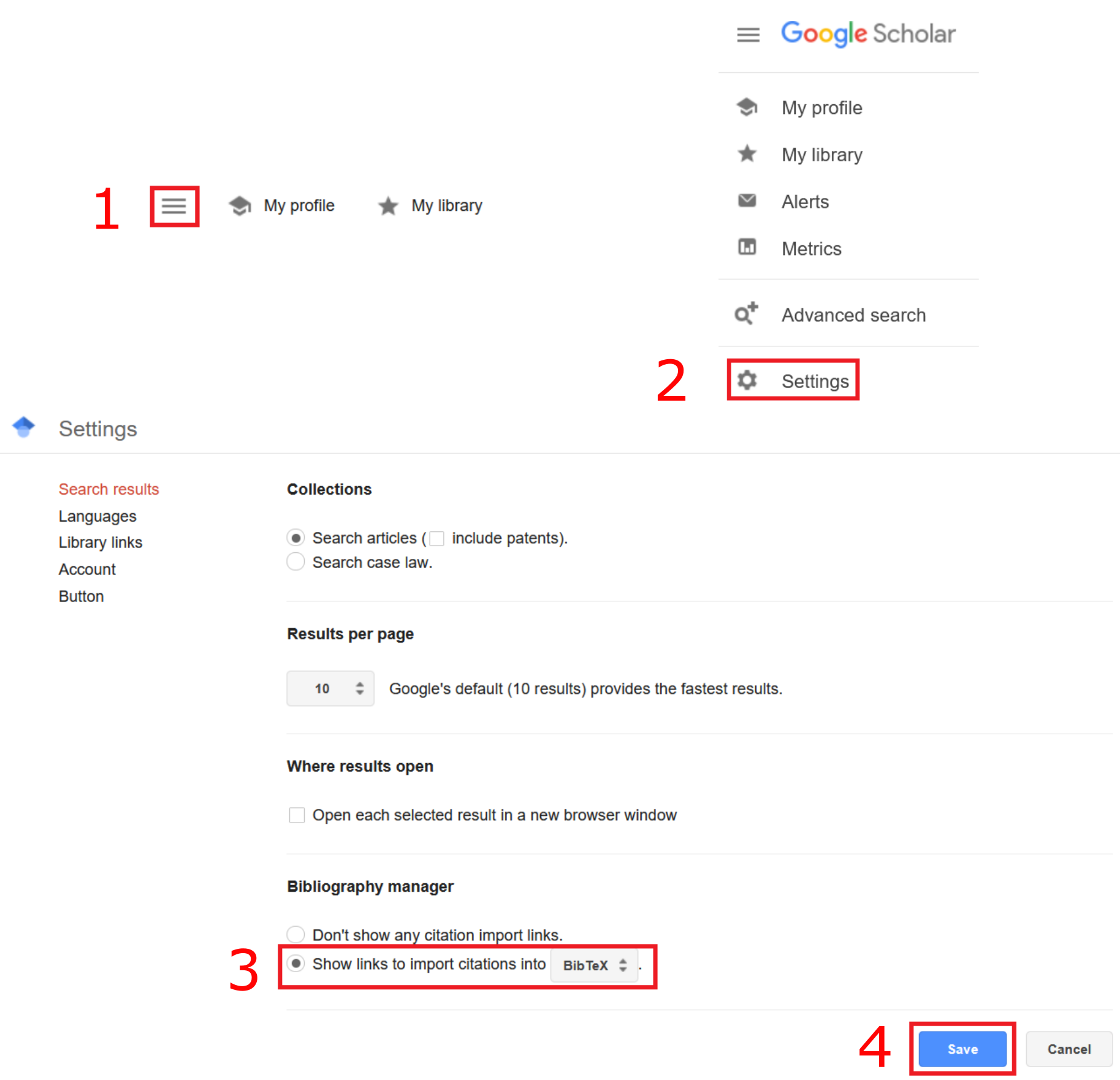
Figure 11.13: Enable BibTeX in Firefox 106.0.1

Browser versions may vary. For assistance, refer to the discussion forum if needed.

2. Export BibTeX Entries: After enabling BibTeX export, a new link “Import into BibTeX” will appear in Google Scholar (see Fig. 11.14).

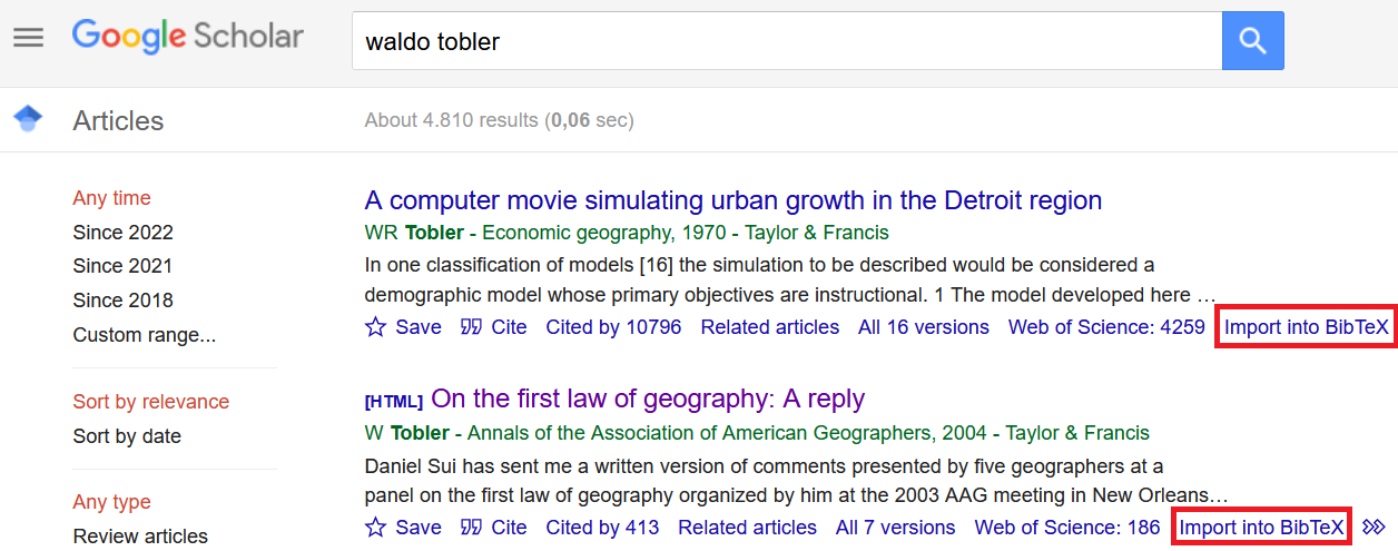
Figure 11.14: BibTeX Link in Firefox 106.0.1

Click the link and copy the BibTeX code into your .bib file.

3. Integrate References in RMarkdown: Specify the location of your .bib file in the YAML metadata of your RMarkdown document (bibliography: <.bib file>). Insert @ followed by the BibTeX key to add citations (see Fig. 11.15).

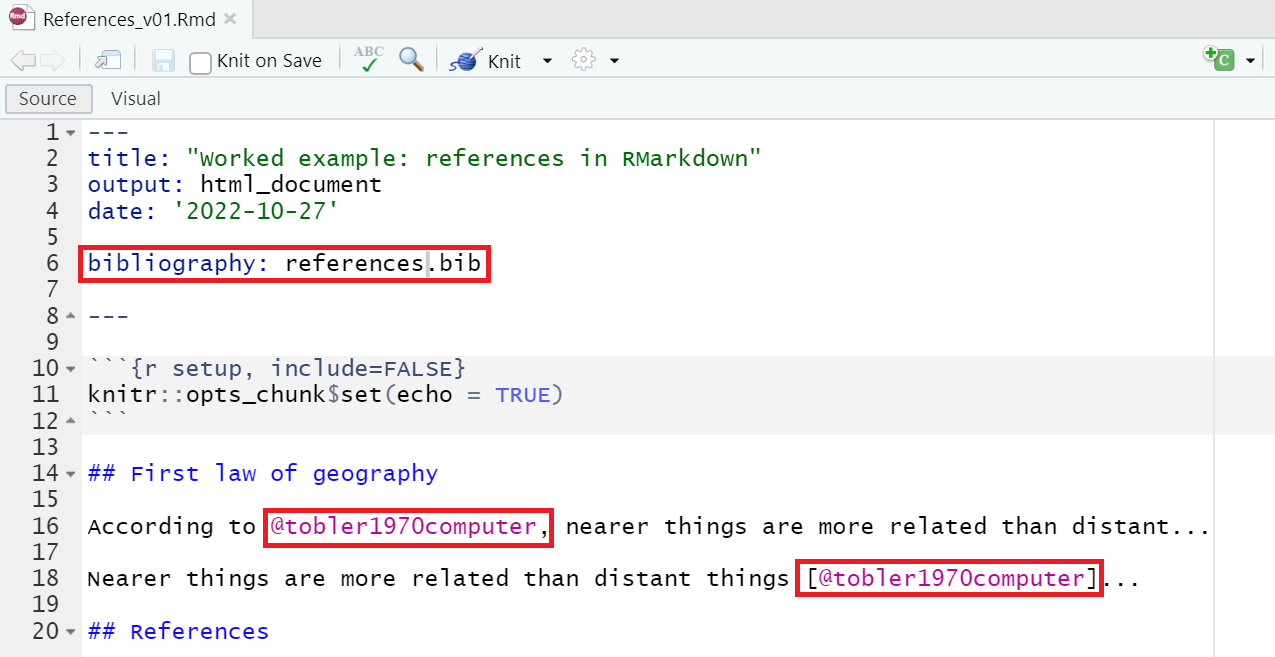
Figure 11.15: Integrate BibTeX reference in RMarkdown document

4. Compile the Document: Knit the R Markdown file as HTML, PDF, or Word. The rmarkdown package processes both indirect (without square brackets) and direct citations (with square brackets) and includes a bibliography (see Fig. 11.16).

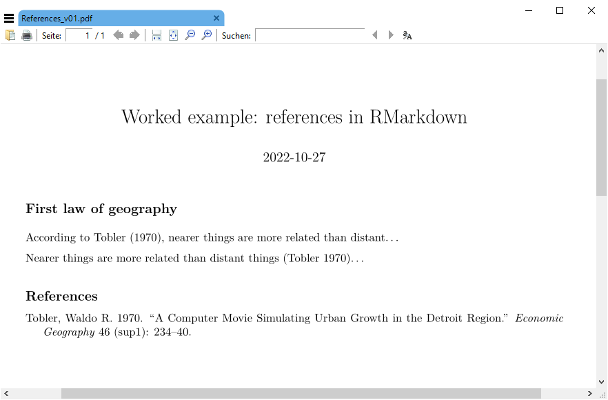
Figure 11.16: Knit R Markdown as PDF

For a practical demonstration, download and explore this RMarkdown reference example. Unzip the folder and open the .Rproj file in RStudio.

Explore more RMarkdown syntax examples in the RMarkdown Cheatsheet.

11.6 Speed up your workflows

R Markdown significantly enhances the efficiency of repetitive workflows. For instance, consider a scenario where a client requires daily updates on specific spatial economic indicators. Instead of manually generating a new report each day, R Markdown can automate this process, creating data reports with charts that update automatically upon compilation. This approach can save substantial time and effort.

Real-time data retrieval is possible through Alpha Ventage, which provides financial market data via the Alpha Ventage Rest API. The R library alphaventager facilitates API access within R. The use of alphaventager enables the extraction of various types of financial data, including real-time stock prices, FX rates, and technical indicators, directly into R. This allows for efficient data processing and visualization, making it a good tool for finance-related reports and analyses in R Markdown.

Explore a practical example by downloading this draft finance data report. Unzip the folder and open the .Rproj file in RStudio.

The project includes:

• A .bib file with a BibTeX reference.
• A .csv file in the data folder, listing over 400 country names, national currencies, and currency codes.
• An .Rmd file with inline R code that renders real-time currency exchange rates in a map.

Review the .Rmd file thoroughly before compiling an HTML output. Note that it includes an interactive Leaflet map, making HTML the only supported output format.

Try enhancing the report with an additional spatial indicator, such as a map displaying exchange rates from national currencies to the Euro.

11.7 Self-study

The vast functionalities of R Markdown extend beyond the scope of a single lesson. To fully exploit its capabilities, refer to the comprehensive online book R Markdown: The Definitive Guide.

This guide covers additional topics such as Notebooks, Presentations, support for languages like Python, C++, SQL, and more complex document creation with extensions like BookDown or ThesisDown. While R Markdown predominantly supports R, its flexibility extends to integrating other programming languages like Python, C++, and SQL. This integration is facilitated through specific settings in the code chunks of the R Markdown document. For instance, by specifying the python engine in a code chunk (e.g., {python}), you can seamlessly run Python code within your document. Similar approaches are used for C++ (using the cpp engine) and SQL (using the sql engine). These capabilities are enabled by the knitr package, which supports various languages, allowing for a multi-language analytical workflow within a single R Markdown document. Experimenting with these various features is key to mastering R Markdown.

Fun Fact: This module was written using BookDown.