10  Movement

In this lesson, we will look into the fascinating field of modelling agent movement. Smart agents move to pursue a purpose, while dynamically adapting their movement to dynamically changing environments. The emerging spatio-temporal patterns of landscape-agent interactions unveil the dynamic nature of process - pattern relations: individual-level behaviour causes patterns at landscape level, and at the same time it is the configuration of landscapes that shape local processes of agents. The second part of this lesson looks into social movement, where agents adapt their movement to each other and thus can generate intriguing social movement patterns.

Learning Objectives

Upon completion of this lesson, you will be able to

• build models with random and with purposeful movement,
• implement models in which agents interact with the landscape, and with other agents, and
• design social movement models following decision-making concepts.

10.1 Random walk

We start with the simplest type of movement ‘random walk’, which we already discussed in this model before. It is often used as reference model to quantify the effect of more mechanistic models that simulate a particular movement process. In Figure 10.1, you can see the random walk pattern of five agents after 500 time steps. At each time step the direction is defined randomly between 0° and 359° and the step length is one unit. Although it is fairly unrealistic that a living agent moves completely randomly, it is commonly used in models where the underlying intention of movement does not matter or is not known.

Figure 10.1: Random walk assumes a completely random choice of direction each time step.

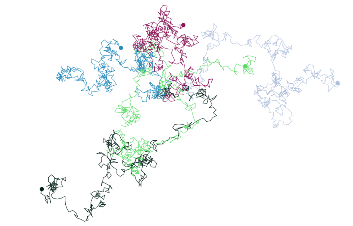
Random walk emerges into an interesting spatial pattern. The Euclidean distance that a random walker moves away from its starting point can be described mathematically: the root mean square (RMS) of the distance to the starting point equals the step length (L) times the square root of the walk duration, i.e. the number of steps (t):

\sqrt(R^2)=L\sqrt(t)

You are well acquainted with the GAMA code for random movement by now:

// random walk
do wander;

10.1.1 Correlated random walk

Correlated random walk restricts the turning angle at a single time step, for example to just +/- 30°. The result is a more persistent movement. However, it still is random movement: for correlated random walk the same mathematical relation between the number of steps and the distance to the starting point emerges at a broader scale.

We have used correlated random walk before:

// correlated random walk
do wander amplitude: 60.0;

Another variation would be to introduce some randomness into step lengths. To make a model (appear) more realistic the modeller can fit the distribution of observed step lengths and turning angles to the random walk behaviour.

Here is the GAMA code, making use of the gauss function, which takes the mean and the standard deviation as parameters:

// correlated random walk with normally distributed, random variation in turning angles and step lengths
do wander speed: gauss(1.0,0.3) amplitude: gauss(60.0,10.0);

10.1.2 Lévy flights

Another useful random movement representation is to apply a skewed distribution to step lengths. Figure 10.2 shows the movement pattern that emerges, if an agent usually walks around with small steps, but sometimes “jumps” over larger distances. Lévy flights for example represent a human taking a flight, or an invasive species being transported over large distances that exceed its natural movement abilities.

Figure 10.2: Lévy flights are like random walks except for their step length, which follows a distribution with a heavy tail.

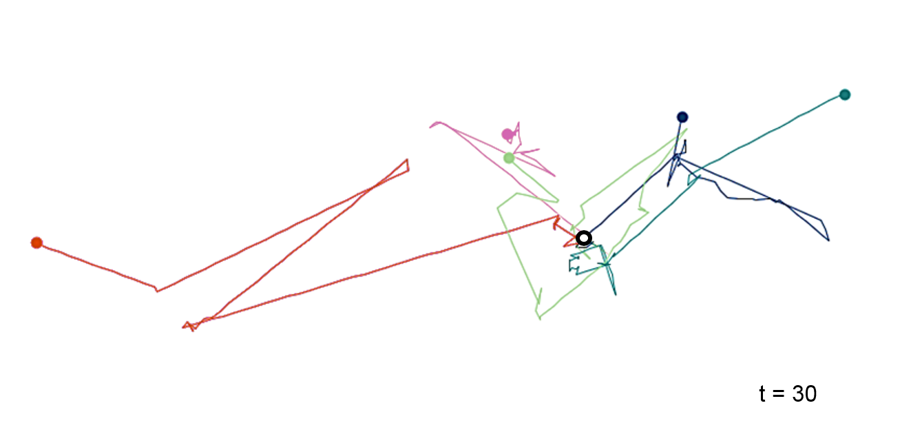
The term Lévy flights was coined by Mandelbrot (1982) in his highly impactful book on “The fractal geometry of nature” to honour Paul Lévy, who has first implemented a skewed distribution of step lengths.

To implement Lévy flights in GAMA, you can use the skew_gauss function with the following parameters: min value, max value, clusteredness of values, and the skew direction, where negative values are skewed towards the min and positive values towards the max value.

// Lévy flights
do wander speed: skew_gauss(0.0, 1.0, 0.7, -2);

Random walk and its derivatives show a pattern that might look like a pattern that we encounter in the real world, but these models do not represent the mechanism of this movement. Or to use the correct terminology: random walk models are phenomenological, not mechanistic.

10.2 Moving with a purpose

The real strength of ABMs unfolds if processes are represented in a mechanistic way, so that the modeller can gain a clear understanding of the interrelation between behaviour and emerging spatio-temporal patterns. The representation of agents that move through space following their specific, individual purpose is the core idea of agent-based models.

Movement is not an end in itself, but it is an activity that serves some purpose. Purposeful movements thus are motivated by a goal on what to achieve. To represent purposeful movement in a model, this goal needs to be made explicit. A number of skills may be necessary to achieve the goal: identification of a sensed or memorised target that helps to fulfill the goal, a spatial memory of the location of relevant objects in the landscape, path memory and related walking strategies, such as self-avoiding walk (to avoid just ‘harvested’ sites) or reinforced walk (to revisit sites that have been rich in resources).

In GAMA, there are two movement commands with which purposeful movement can be represented: goto target: {point} and move heading: (degrees). Remember that the direction in GAMA is a bit weird: 0° isn’t North, but East.

Let’s start and model an agent to go west, so the heading should be 180°:

    reflex moveWest {
        do move heading: 180.0;
    }

Alternatively, you can use the goto command to head towards a specific target. This can be a stationary item, or even a moving target.

    reflex gotoTree0 {
        do goto target: tree[0].location;
    }

However, note that goto doesn’t allow to define bounds for the movement. For example, you cannot force the agent to stay within e.g. a forest geometry. To move towards a target within the bounds of a geometry, you can make use of the move statement, together with towards and bounds:

    reflex moveToCow0 {
        do move heading: self towards cows[0] bounds: pasture_geometry;
    }

10.3 Moving in landscapes

We are now equipped to look into the interaction between an agent and a cellular automaton. The agent moves through the landscape in order to pursue its goal. According to the ABM decision-making workflow, in each time step each of the agents scans its neighbouring cells of the CA (Figure 10.3), listens to its inner states, decides what to do according to its behavioural rule sets, and then takes action.

Figure 10.3: The cow agent scans its local neighbourhood for the best grazing spot.

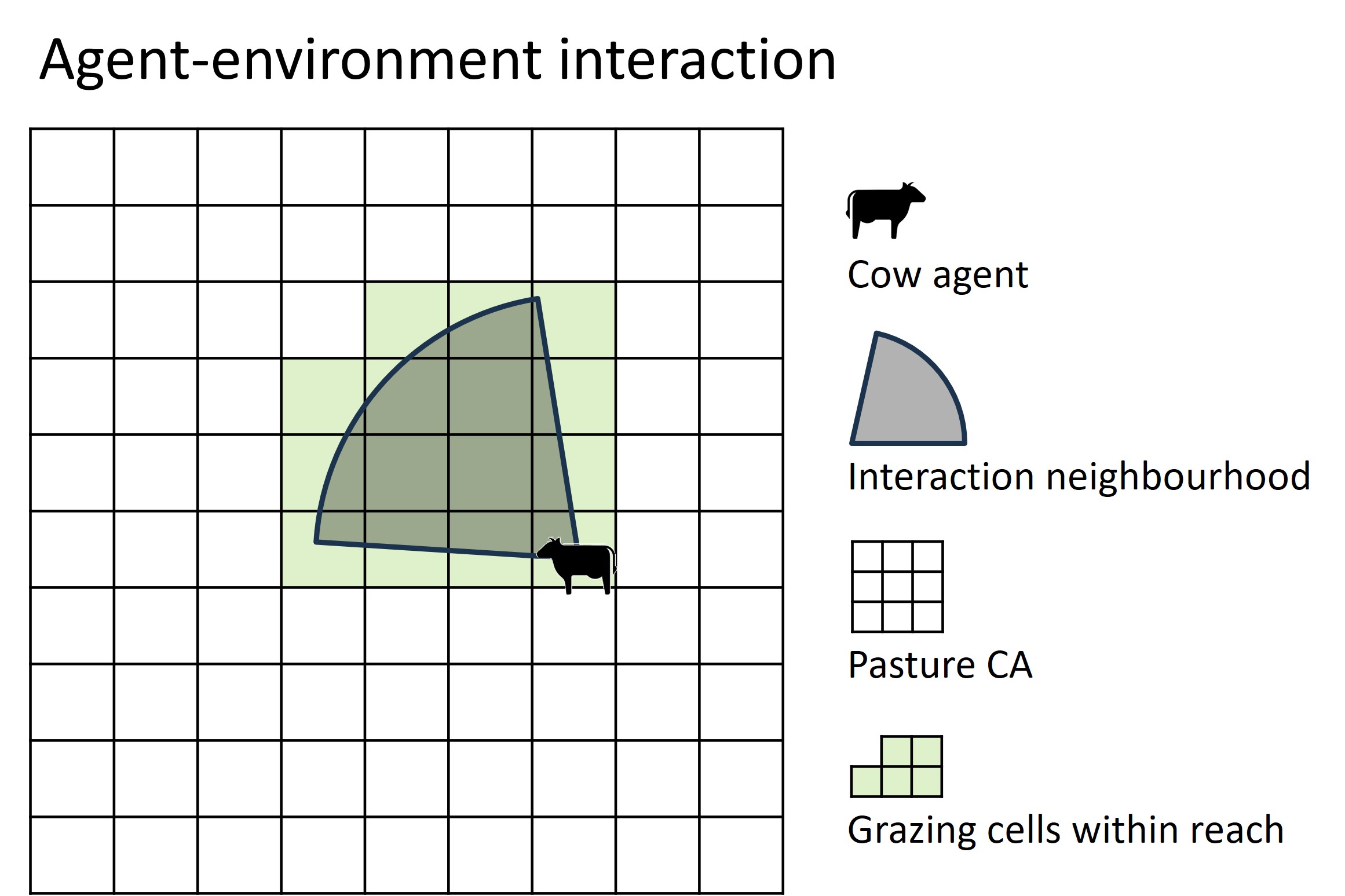
Operationally, the subset of potential grazing cells of the grassland CA are identified with an overlay operation of the cow’s action area with the CA grid. Let’s assume that the action area of a cow is a simple circular buffer:

grassland at_distance range;

More generally, assuming the action area is a cone, a viewshed or any other geometric shape, we can write:

grassland intersecting cow_action_area;

Now, there comes the “trick” to implement interaction in the GAMA model code. In the cow agents, we declare a list of type grassland (which is the CA in the cattle-pasture example). To this list variable we assign the grassland cells within reach (or within vision) of each cow at each time step, so that each cow “owns” the grazing cells it can reach (or see):

// cow agents
species cows skills: [moving] {
    //declare (initially empty) subsets of grassland cells
    list<grassland> my_grassland_cells;
    list<grassland> visible_grassland_cells;

    reflex update_interaction_neighbourhood {
      //action area
      my_grassland_cells <- grassland at_distance range;
      //perception area
      visible_grassland_cells <- grassland at_distance vision;
    }
}

Finally, the cow moves randomly to a spot within the action area:

do goto target: one_of my_grassland_cells;

Alternatively, we can implement purposeful movement to the grassland cell within reach that has the highest biomass:

best_spot <- my_grassland_cells with_max_of (each.biomass);
do goto target: best_spot ;

Even more sophisticated, cows can perceive a larger area than they can reach in one time step. They identify the best grass and start to walk there:

my_grassland_cells <- grassland at_distance vision;
best_spot <- my_grassland_cells with_max_of (each.biomass);
do goto target: best_spot speed:range #m/#s ;

Exercise: ABM-CA interaction

The code below defines the subset of cells of an action neighbourhood within range. In the last line of code, the goto target is again limited to a maximum speed of “range”. This seems to be redundant. Can you think of a reason, why it nevertheless could make sense to limit the movement?

    reflex graze {
        my_grassland_cells <- grassland at_distance range;
        best_spot <- my_grassland_cells with_max_of (each.biomass);
        do goto target: best_spot speed:range #m/#s ;

Check the answer.

The buffer overlay operation grassland at_distance range selects all cells intersecting (= fully or partly covering) the circular range of the cow. If the cow just goes to the best_spot cell, it would move in the raster topology, i.e. go to the centre of the target cell. However, the cell centre potentially could be located outside the buffer (see also Figure 10.3), so that it makes sense to limit the movement distance.

Check the online documentation for further information on spatial operators in GAMA.

In the following exercise, we will implement a full model that represents interaction between cattle and grassland.

Exercise: pasture - cattle interaction

This exercise builds on the “Geosimulation pasture model”, which was the last exercise in Lesson 4 “Models of spatial systems”, where we combined the CA of a pasture with moving cattle. In the Geosimulation pasture model, cows run around the pasture, but there is no interaction between cattle and the grassland. The objective of this exercise is to let cows feed grass on the pasture, win energy and locally reduce the grass biomass.

Instructions

• open the Geosimulation pasture model and save it under a new name
• add a global variable for the range of the cows (=action radius)
• add an agent variable for a cow’s energy level.
• add an agent variable with the grassland cells within reach
• represent purposeful movement directed to the pasture cell within range that has most grass
• remove grass and gain energy

Optionally, you can play around with the parameters and number of cows to find the maximum number of cattle that the pasture sustains under given circumstances.

View the model code.

/***
* Name: Ex L8a_interactive CA-ABM
* Author: WALLENTIN, Gudrun
* Tags: agent movement, interaction with a landscape
* Description: model in the "Spatial Simulation" module of the UNIGIS curriculum
***/

model ExL8a_interactive_CA_ABM

global  {

    //Load geospatial data
    file study_area_file <- file("../includes/study_area.geojson");
    //fenced area includes shrubs and grassland
    file fenced_area_file <- file("../includes/vierkaser.geojson");
    //high-quality pasture area
    file lower_pasture_file <- file("../includes/lower_pasture.geojson");
    //low-quality pasture area
    file hirschanger_file <- file("../includes/hirschanger.geojson");

    //grass regrowh rate
    float grass_growth_rate <- 0.008;

    //Define the extent of the study area as the envelope (=bounding box) of the study area
    geometry shape <- envelope (study_area_file);

    //extract the geometry from the vector data
    geometry fence_geom <- geometry(fenced_area_file);
    geometry lower_pasture_geom <- geometry(lower_pasture_file);
    geometry hirschanger_geom <- geometry(hirschanger_file);
    geometry pasture_geom <- lower_pasture_geom + hirschanger_geom;

    //the action neighbourhood (range) of a cow in one time step, i.e. its potential speed
    float range <- 10.0;

    //Create the agents
    init {
        //create 5 cow agents that are located within the pasture
        create cows number: 15 {
            location <- any_location_in (pasture_geom );
        }
        ask grassland {
            color <- rgb([0, biomass * 15, 0]);
        }
    }
}

// cow agents
species cows skills: [moving] {
    float energy <- 5.0;
    //declare a (initially empty) subset of grassland cells
    list<grassland> my_grassland_cells;
    //declare a grassland cell variable to hold the spot with the best grass within reach
    grassland best_spot;

    //behaviour: move to a yummieh grassland spot
    reflex graze {
        my_grassland_cells <- grassland at_distance range;
        best_spot <- my_grassland_cells with_max_of (each.biomass);
        if location = best_spot.location {
            do wander amplitude: 60.0 speed: range #m/#s;
        }
        else {
            location <- best_spot.location ;//speed:range #m/#s ;
        }
        energy <- energy - 1;
        ask grassland closest_to (self)  {
            if biomass > 4 {
                biomass <- biomass - 4;
                myself.energy <- myself.energy + 1.2;
            }

            else if biomass < 0 {
                biomass <- 0.0;
            }
        }
    }

    //visualisation
    aspect base {
        draw circle (5) color: #lightblue;
    }
}

//The cellular automaton represents the grazeland
grid grassland cell_width:5 cell_height:5  {
    float biomass;
    float max_biomass <- 0.0;

    init {
        //assign the value of 1 as the max. biomass within the fenced area
        if self overlaps(fence_geom){
            //set the maximum biomass of a grazeland cell to 1
            max_biomass <- 1.0;
            biomass <- max_biomass;
        }
        //if the cell overlaps the lower pasture: assign the value of 10 to the biomass (this overwrites the biomass=1 within the fenced area)
        if self overlaps(lower_pasture_geom){
            max_biomass <- 10.0;
            biomass <- max_biomass;
        }
        //if it is not in lower pasture, but it overlaps Hirschanger: assign the value of 7 to the biomass ("else if" overwrites the fenced area, but not the lower pasture)
        else if self overlaps(hirschanger_geom){
            max_biomass <- 7.0;
            biomass <- max_biomass;
        }
    }

    // let grass grow until its maximum potential
    reflex grow_grass when: max_biomass > 0 {
        //logistic growth: N + r*N*(1-N/K)
        biomass <- biomass + grass_growth_rate * biomass * (1 - biomass / max_biomass);
        color <- rgb([0, biomass * 15, 0]);
    }
}

//Simulation
experiment virtual_pasture type:gui {
    output {
        display map type: opengl{
            //draw the geometry of the pasture
            grid grassland;
            species cows aspect:base;
        }
        display chart type: 2d{
            chart "mean energy" {
                data "energy of cows" value: mean(cows collect each.energy);
            }
        }
    }
}

10.4 Social movement

Social movement is the adaptive movement of agents in response to other nearby agents, which involves attraction, repulsion and imitation (alignment). Social movement results in emergent patterns, like the dispersed patterns of people in a subway train, who reorganise to maximise their distances after each stop, or the clustered movement of schooling fish (Figure 10.4).

Figure 10.4: The pattern of a school of fish swimming together emerges from social movement behaviour.

The principle of modelling interactive social movement, is similar to modelling movement of agents in a dynamic CA environment: the spatial configuration establishes which agent will adapt its movement to which other agents. Consider the cow agents in Figure 10.5 with their respective neighbourhoods: who will adapt its movement to whom?

Figure 10.5: Four cow agents and their neighbourhoods. Cow C will adapt to cow B, and cow D will adapt to cows C and B. Cows A and B do not perceive any other cows in their neighbourhoods and thus they exhibit no adaptive behaviour.

Let’s consider the example of flocking for the following exercise on social agent movement.

Exercise: social cow movement

This exercise implements interactive flocking movement of cows following the decision-making template: perceive - decide - act.

1. Perceive

First, we declare a list-variable of type cows to represent the agents to interact with. To this list-variable we assign the cows within the perception neighbourhood, so that each cow “owns” the cows it can perceive at a particular time step. Further, the cows also perceive their nearest neighbour.

// cow agents
species cows skills: [moving] {
  geometry perception_neighbourhood;
    //declare an (initially empty) subset of cow agents
    list<cows> flockmates;
    cows nearest_neighbour;

    reflex perceive {
        perception_neighbourhood <- arc(vision, heading, vision_angle);
        // search for flockmates
        flockmates <- ((cows overlapping perception_neighbourhood) - self);
        if (not empty (flockmates)) {
            nearest_neighbour <- flockmates with_min_of(distance_to (self.location, each.location));
        }
    }
}

2. Decide

According to the decision-making sequence, the agents next decide what to do. In the NetLogo implementation of the flocking model, the behavioural decisions that lead to flocking are described as follows:

• If my nearest neighbour is too close: turn away,
• otherwise align with the average heading of my flockmates, and
• turn towards them.

The following code translates this decision-making blueprint into GAMA code. Working your way through the code, you will see some actions that are called with a do xxx command. These actions are not included in the code segment below in order to concentrate on the important parts. However, if you are curious, you will find the full code at the end.

    // make decisions according to the behavioural blueprint for flocking
    reflex decide {

    // if there are other agents in vision...
        if (not empty (flockmates)) {
          // and my nearest neighbour is too close: turn away
            if (distance_to (self, nearest_neighbour) < min_separation) {
                do separate;
                action_neighbourhood <- arc(step_length, heading, max_separate_turn);
            }
            // otherwise align and cohere
            else {
                do align;
                do cohere;
                action_neighbourhood <- arc(step_length, heading, max_align_turn + max_cohere_turn);
            }

        // if there are no other agents in vision: turn a bit to prepare random walk
        else {
            do prepare_random_walk;
            action_neighbourhood <- arc(step_length, heading, max_random_turn);
        }
    }

3. Act

Finally, following the decision that each of the cows took, the agents then execute the action. In the flocking model, the turns are implemented as part of the decision-making, so that the action is limited to moving into the given direction:

reflex act {
    // ..and move into the new direction
    do move speed: step_length;
}

To explore the model in operation and to check the helper procedure and other details, you can download the full GAMA flocking model.

10.5 Mixed movement

In reality, animals do several things at the same time. They stick together in a herd while they graze good grass spots. The following exercise combines these movements into one model:

Exercise: mixed movement

The mixed movement model integrates the models of the two previous exercises (Ex L8a_interactive CA-ABM and Ex_L8b_flocking_interaction.gaml) by splitting each simulation step into two sequential phases. These phases are scheduled globally so that all cows complete first the grazing phase before any cow begins with the flocking phase. After each phase the cows move half the step length. This way, grazing and flocking is weighted equally.

To explore the model in more depth, you can download the full GAMA model.

References

Mandelbrot, Benoit B. 1982. The Fractal Geometry of Nature. Vol. 1. WH freeman New York.