5%/%2[1] 2This module will equip you with fundamental R programming skills, beginning with core programming concepts common to most languages. These include Datatypes, Operators, Variables, Functions, Control Structures, and Libraries. You will gain a solid understanding of these basics, forming a strong foundation for advanced programming.
We then progress to more complex data types like Data Frames and Tibbles, and explore how to Read and Write both spatial and non-spatial datasets. Special emphasis is placed on techniques to manipulate data, enabling you to adeptly manage and analyze datasets. This will be particularly useful for preparing and refining data for in-depth analysis.
The module also focuses on data visualization, where you’ll learn to create informative and compelling visual representations, such as box plots, scatterplots, line plots, and maps. These skills are critical for data exploration and presenting your findings in an accessible manner.
Additionally, the course introduces the essentials of working with spatial data. This includes handling spatial data structures, performing spatial data manipulation, and understanding spatial relationships.
Upon completing this module, you’ll possess foundational R programming skills, preparing you for more advanced topics such as “Geospatial Data Analysis”, as covered in the “Spatial Statistics” module of the MSc program.
This module partly draws from granolarr, developed by Stef de Sabbata at University of Leicester. For further exploration, refer to the Webbook R for Geographic Data Science. We particularly recommend its chapters on Statistical Analysis and Machine Learning for those interested in advanced R applications.
R is versatile in data science and analytics, with applications including:
Why R stands out:
R, a high-level programming or scripting language, relies on an interpreter instead of a compiler. This interpreter directly executes written instructions, requiring adherence to the programming language’s grammar or Syntax.
In this lesson we will focus on some key principles of the R syntax and logic.
Before you can run your code, you have to install R together with an Integrated Development Environment (IDE) on your machine:
The IDE is where you write, test, and execute your R programs, we strongly recommend using RStudio Desktop, which is freely available for download.
This video offers a concise RStudio overview Figure 1.1:
Encounter technical difficulties? Please consult the discussion forum!
With RStudio and R installed, let’s dive into coding. The Console Window in Figure 1.2 is where the interpreter outputs results based on your input.
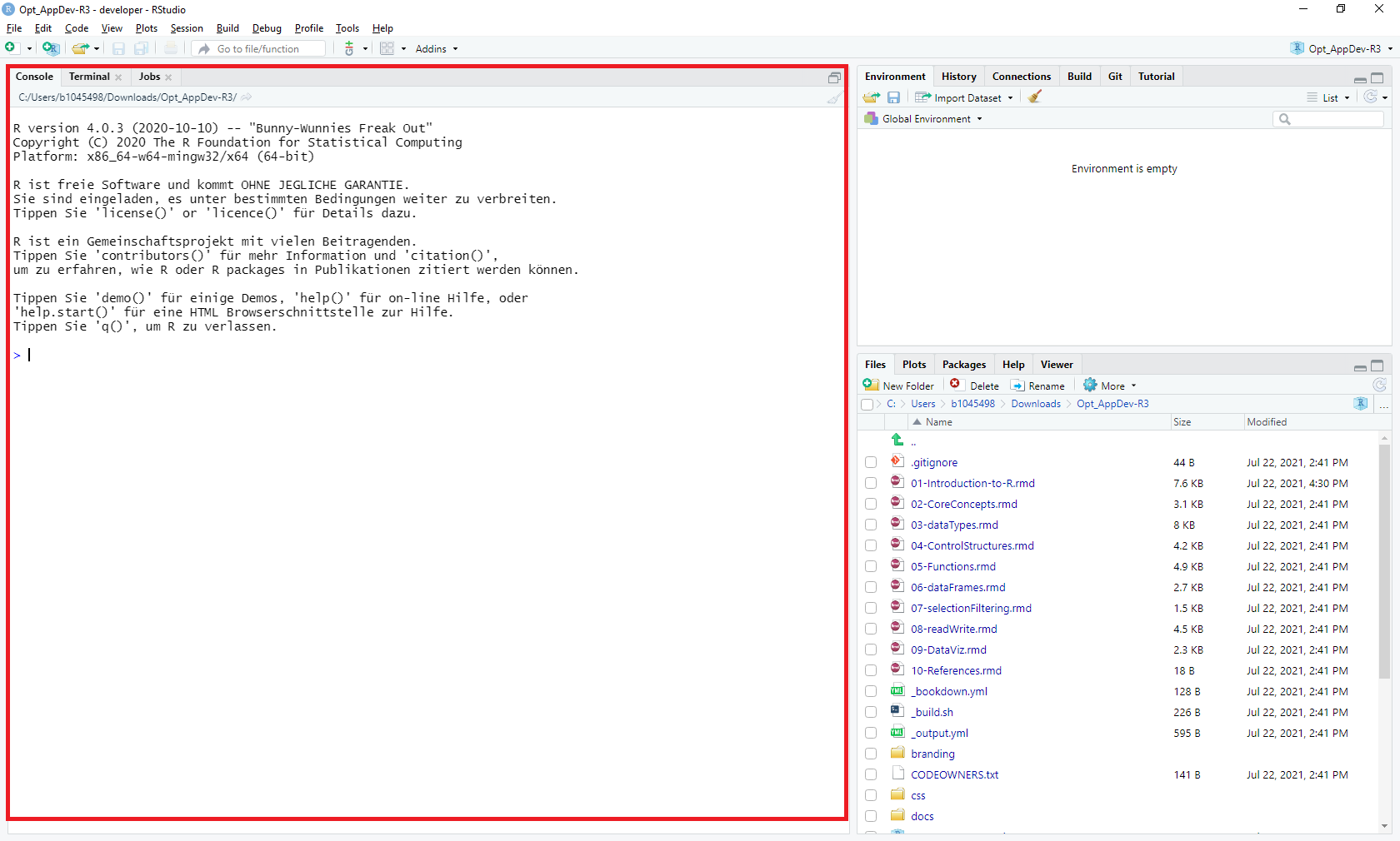
Type in a numeric value (e.g., 3) and press Enter. The interpreter returns the input value preceded by a bracketed number. The value in brackets indicates that the input is composed of one single entity.
What happens when you input a text value (e.g., ‘test’)?
The interpreter returns an error when unquoted text is entered, as it’s not recognized as a string. In R, text or strings must be enclosed in quotes (either single 'test' or double "test") to be understood as character data. Text is commonly referred to as String or String of Characters.
If you start your input with a hash symbol (#) the interpreter will consider that line as a comment. For instance, if you type in # Test Test Test, you will see that nothing is returned as an output. Comments are extremely important as they allow you to add explanations in plain language. Comments are fundamental to allow other people to understand your code and it will save you time interpreting your own code.
R’s simple data types, essential for encoding information, include:
TRUE or FALSE valuesLogical TRUE or FALSE values are typically the result of evaluating logical expressions.
Together these three simple data types are the building blocks R uses to encode information.
If you type a simple numeric operation in the console (e.g. 2 + 4), the interpreter will return a result. This indicates that operations (e.g. mathematical calculations) can be carried out on these types.
Logical operations return values of type logical. What value is returned in the console when you type and execute the expression 2 < 3?
The interpreter returns TRUE, because it is true that 2 is less than 3.
R provides a series of basic numeric operators:
| Operator | Meaning | Example | Output |
|---|---|---|---|
| + | Plus | 5 + 2 | 7 |
| - | Minus | 5 - 2 | 3 |
| * | Product | 5 * 2 | 10 |
| / | Division | 5 / 2 | 2.5 |
| %/% | Integer division | 5 %/% 2 | 2 |
| %% | Modulo | 5 %% 2 | 1 |
| ^ | Power | 5^2 | 25 |
Whereas mathematical operators are self-explanatory, the operators Modulo and Integer division may be new to some of you. Integer division returns an integer quotient:
5%/%2[1] 2Note: The code above returns a value of 2. The number in squared brackets [1] indicates the line number of the return.
Execute 5 %% 2 to test the ‘Modulo’ operator.
The “Modulo” returns the remainder of the division, which is 1 in the example above.
R also provides a series of basic logical operators to create logical expressions:
| Operator | Meaning | Example | Output |
|---|---|---|---|
| == | Equality | 5 == 2 | FALSE |
| != | Inequality | 5 != 2 | TRUE |
| > (>=) | Greater (or equal) | 5 > 2 | TRUE |
| < (<=) | Less (or equal) | 5 <= 2 | FALSE |
| ! | Negation | !TRUE | FALSE |
| & | Logical AND | TRUE & FALSE | FALSE |
| | | Logical OR | TRUE | FALSE | TRUE |
Logical expressions are typically used to execute code dependent on the occurrence of conditions.
What logical values are returned by the following expressions:
Type and execute these expressions in the RStudio console to validate your assumptions.
Apart from Stef de Sabbata’s teaching materials, this module draws from various sources, most of which are available online: