Lesson 7 Spatial processes
Whereas traditional simulation models in the early days of computers were (had to be..) simple and highly abstract models, today’s models often aim to be much more realistic. Today, many models attempt to simulate a certain study area in order to address and solve a specific real-world problem. The increasing computer power has opened a lot of possibilities for the fruitful application of simulation modelling in many domains. However, the realism sometimes obscures the underlying spatial processes. To better interpret the behaviour of complex simulation models, it often helps to understand the behaviour of simple models. We can assume that at the core of the today’s increasingly complex ‘realistic’ models there is only a limited set of underlying processes. O’Sullivan and Perry (2013) argue that there are not more than just three process categories: 1) Aggregation / segregation, 2) Diffusion / spread, and 3) Movement.
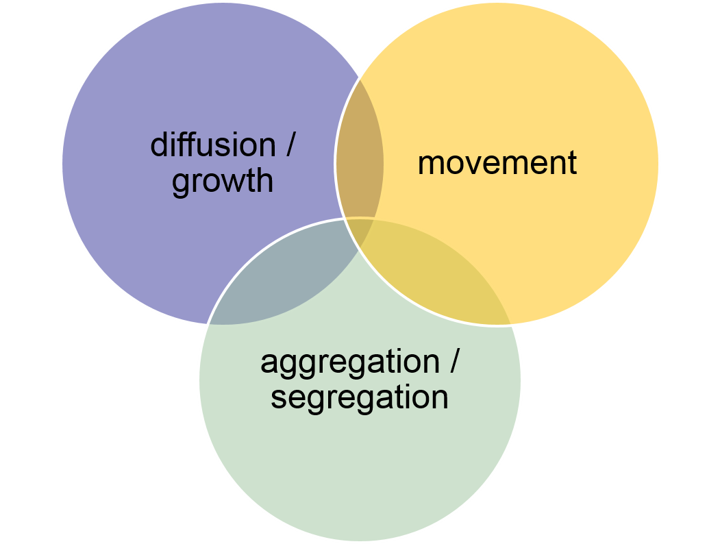
Figure 7.1: Every spatial process can be composed from the three basic processes: diffusion / growth, aggregations / segregation, and movement.
In this lesson we will discuss the three ‘building block models’ that generate these processes, following the structure and examples provided by O’Sullivan and Perry (2013). Please refer to this book for further details: it is excellent reading! Also you can find further materials on the book’s supporting website: Pattern & Process with a lot of toy models that implement the discussed process types (unfortunately coded in NetLogo). Together with a UNIGIS uLecture presentation by David O’Sullivan these are great resources to dig deeper.
In the module, we will first explore the behaviour of abstract and seemingly simple models from a conceptual, generic perspective and then we will look into typical application areas. We will also see, that the three processes cannot always be strictly separated, but it is still a good way to structure typical modelling principles.
7.1 Aggregation and segregation
Aggregation and segregation are closely related processes. Whereas aggregation refers to the process of spatial clustering of one type of entity (e.g. the herding process of animals in a population), segregation refers to the process in which different types of entities separate (e.g. on a beach gulls stay near other gulls and seals rest next to other seals). If the initial distribution of two populations is randomly distributed in space, then the aggregation of one entity will entail a segregation process: the gathering of seals on the beach automatically entails separation between the gull and the seal population. Simply put, aggregation and segregation are the processes that follow Tobler’s first law of geography: more related things tend to cluster together, which leads to a segregation of dissimilar things. The result of such processes is a heterogeneous, non-random and clustered (=patchy) world.
From a simulation modelling perspective we look at models that generate patchy patterns of spatially extended phenomena. As we have seen in the previous lessons, the most adequate modelling approach to simulate processes of spatially extended phenomena are cellular automata. Further, we will consider an alternative approach, in which patchy patterns result from a top-down process. We might also look at aggregation processes that result from movement of individual entities, like the flocking of birds. However, this process will be discussed later, together with other processes that explicitly involves movement of individual agents.
7.1.1 Asynchronous CA update
In a cellular automaton usually all cells are updated at each time step according to the transition rules, whereas in an asynchronous model, only one random cell is updated per time step. Let’s have a closer look at the sort of processes that can be generated by such models. A simple model to start with is called ‘contact process’ model. It is a system of binary states that is defined by the following asynchronous update rules:
- If the cell is alive, it will die with some probability.
- If the cell is dead, it will become alive with a probability given by the proportion of living neighbours.
The result is a patchy landscape that dynamically changes its appearance, but establishes at a certain proportion of ‘living’ cells.
Under the same category fall succession models, where these models can take multiple possible states that succeed each other, e.g. grass, bushes and trees. The result is again a dynamically changing, segregated pattern of successional stages of vegetation.
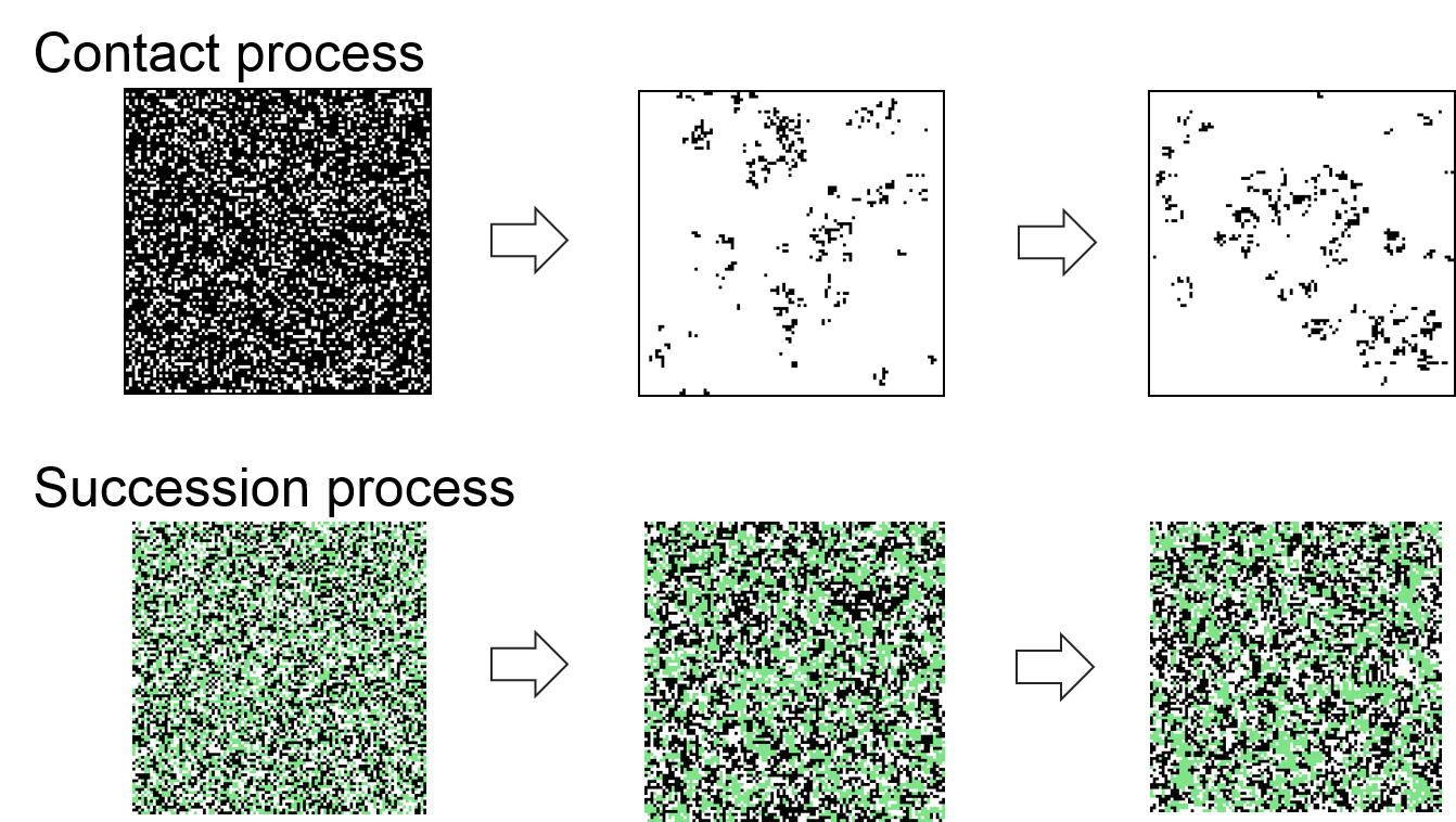
Figure 7.2: CA in which only one random cell is updated per time step result in dynamically changing, segregated pattern.
7.1.2 Shelling’s segregation model
Thomas Schelling’s models of spatial segregation of people with different nationalities in a city (Schelling 1971) are amongst the most influential spatial simulation models. Cells may take three states: vacant, blue and red. The two coloured cells tolerate cells of opposite colour in their neighbourhood, but desire to be surrounded by a minimum proportion of cells of the same colour. If a cell is ‘dissatisfied’ with its current location, it can switch to the closest ‘vacant’ location with a satisfying neighbourhood. Cells are ‘relocated’ until the desired neighbourhood is reached for all cells, or no further vacant spots with a desired neighbourhood exist. Of course, the same idea can be conceptualised as an agent-based model, where only one agent per cell is allowed. The mechanism is the same – and it shows, how closely the two bottom-up modelling approaches of cellular automata and agent-based models are related.
Figure 7.3: Schelling’s segregation model, NetLogo Web
As you probably have seen in the model of Figure 7.3, the outcome of the Schelling model shows an interesting emergent behaviour: the pattern at the final stage shows a much higher segregation than it would be expected from individual preferences. In Figure 7.2, there are two equally strong populations and a vacancy rate of 10%. Both populations desire that at least 60% of their neighbours are like themselves. However, the resulting pattern shows a highly segregated landscape with a mean probability for a cell to have alike neighbours of more than 90%.
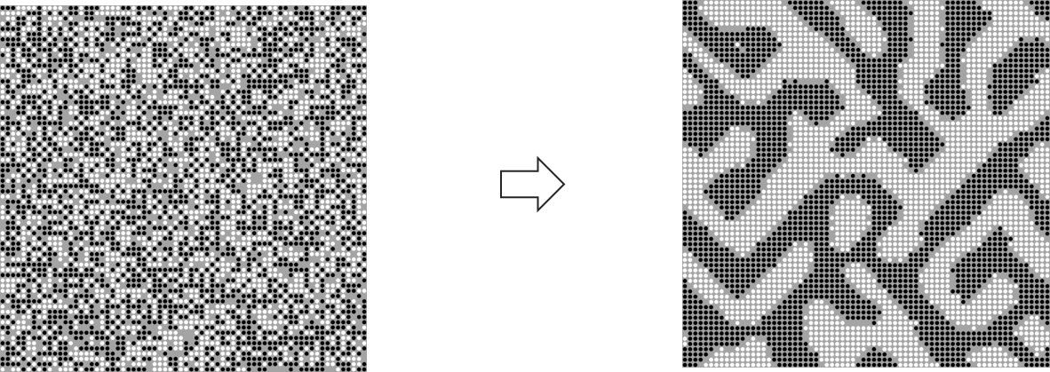
Figure 7.4: CA in which only one random cell is updated per time step result in dynamically changing, segregated pattern.
7.2 Diffusion and growth
There are a few conceptually related processes that all belong to the same family of spatial processes, which describe spread in (heterogeneous) landscapes. Spread is a general term to describe various processes of spatial expansion:
- Diffusion is a random movement of material from regions of high concentration to regions of low concentration.
- Growth has very similar geometric properties. The main difference is that in diffusion processes attribute values get diluted over time, whereas the nature of the growing object stays the same.
- Advection processes describes how something is transported by a moving fluid, e.g. transport of pollutants in a river.
- Finally, percolation describes the movement of a fluid through a porous material. In a wider sense, any process that operates on a heterogeneous (“porous”) surface can be modelled as a percolation process. For example, the spread of a disease through a population, or the spread of a wild-fire through a sparse forest.
7.2.1 Percolation
In simulation modelling, the representation of the ‘porous’ background of a percolation model can be modelled by a grid with loosely occupied cells, or alternatively as linked cells or graphs. From a modelling perspective, the critical part of model design is to find an adequate structure of the porous background. If it is too sparse, percolation will stop after very few steps. If it is too dense, the entire study area will be percolated. The phase transitions at which percolation behaviour change between too sparsely, optimal and too densely occupied grids are very sharp.
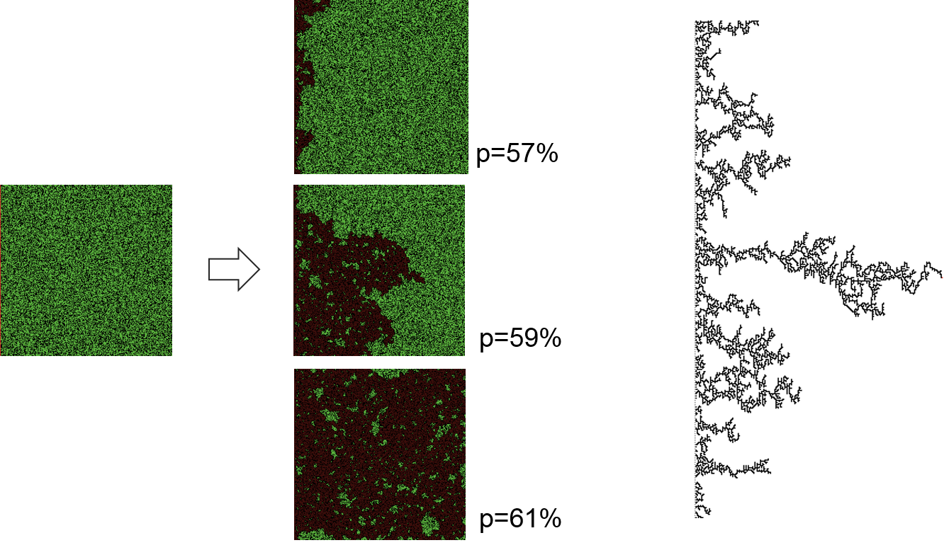
Figure 7.5: Percolation models simulate a spread process through porous environments.
The figures on the left side show a classical example of a percolation model: the spread of a wild-fire. Green cells represent trees in a forest (here: 59% of cells), black cells are not covered by trees. The fire starts from the left side and percolates through the forest until no further trees are in the von Neumann neighbourhood to be ignited. There is a sharp phase transition for the amount of green forest-cells around 59%: at this value, there is a 50% chance that the fire reaches the other side of the forest. This probability sharply drops for a forest density that is only slightly reduced, whereas the entire area gets burned in slightly denser forests.
A modification to ordinary percolation models are invasion percolation models. The heterogeneous background structure in these models is defined by random values that range between 0 and 1. Percolation then works along the lowest value in the neighbourhood. The resulting pattern is shown in the figure on the right side. It resembles the generation of drainage networks.
7.2.2 Eden growth models
The basic way to model growth was suggested by Eden (1961). Therefore, growth models are often addressed as ‘Eden growth models’. The rules of the basic approach are simple:
- Seed an initial site and occupy it
- Randomly select an unoccupied neighbour
- Occupy this neighbour
The emergent pattern of this modelled process shows a compact and dense interior with a diffuse and fringed edge (the actively growing zone). This pattern strongly reminds of growing bacteria, lichen or cities.
Over the time, many variations of this basic model have been made. An interesting variant is the epidemic model (Alexandrowicz 1980) of the spread of a disease: once a new cell is selected to become occupied, it might either turn into the status ‘infected’ or ‘immune’. Similar to percolation models, this epidemic model is very sensitive to the probabilities of being infected vs. being immune upon selection.
Another variant models the spread of invasive species. This model combines local growth with sporadic jumps that occasionally happen after long distance dispersal events. Although such events are rare, they greatly contribute to the rapid spread of invasive species. In Figure 7.6, you can this phenomenon in the example of invasive toads in Austrialia (Phillips and Shine 2004).
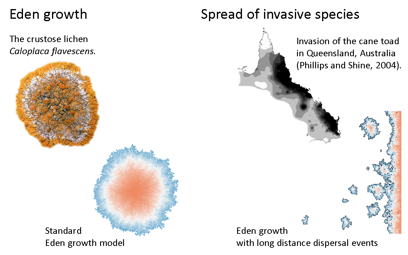
Figure 7.6: Models that simulate biological growth are named after Murray Eden, who first formally described this process.
Exercise: Eden growth
The Eden growth algorithm can be found in almost every cellular automaton. So, let’s have a look, how it can be implemented in GAMA. In this exercise, we will let a forest grow from one central tree. In this case, trees are represented as cells. You can imagine one cell to be inhabited by one tree. So, we have a cellular automaton without agents. In GAMA-specific language that means, we have a grid, but no species.
So the basic structure is as follows:
model EXEdenGrowth

global {
}

grid forest width:100 height:100 {
}
Forest growth is the result of 3 main tree-level processes: seedlings distribution, seed germination and tree growth (and death). We implement these processes as actions and call them from the global section:
model EXEdenGrowth

global {
  reflex forest_expansion {
    ask forest {do distribute;}
    ask forest {do germinate;}
    ask forest {do grow;}
  }
}

grid forest width:100 height:100 {
  action distribute {}
  action germinate {}
  action grow {}
}
We start with the distribution action: if a cell is occupied with a tree, then it will distribute its seeds to all unoccupied neighbours. To accomplish that, we need two boolean grid variables that track whether there is a seedling or a tree on a cell: is_tree and is_seedling. Further, we have the tree age and a maximum age of a tree as cell attributes.
grid forest width:100 height:100 {

    bool is_tree <- false;
    bool is_seedling <- false;
    int treeAge <- -1;
    int maxAge;

    action distribute  {
        if is_tree = true {
            ask neighbors {
                if is_tree = false {
                    is_seedling <- true;
                }
            }
        }
    }
The germination action shall only be executed, if there is a seedling on the cell. It “creates” the tree and all properties, like age and colour.
    action germinate {
        if is_seedling = true and 80 > rnd (100){
            is_tree <- true;
            treeAge <- 0;
            maxAge <- rnd(80,120);
            color <- rgb([0,treeAge * 2,0]);
            is_seedling <- false;
        }
    }
Finally, we let the trees grow if they are below their maximum age, or die otherwise:
    action grow  {
        if is_tree = true and treeAge < maxAge {
            treeAge <- treeAge + 1;
            color <- rgb([0,treeAge * 2,0]);
        }

        if is_tree = true and treeAge >= maxAge {
            is_tree <- false;
            color <- #white;
            treeAge <- -1;
        }
    }
The two last things we are missing, is to plant an initial tree at the beginning (in the global section):
    init {
        ask forest[50,50] {
            is_seedling <- true;
            do germinate;
        }
    }
..and to visualise it by adding an experiment. You are already familiar with this last step. Compile everything together and check, whether your forest grows! Watch the waves of aging forest. After 400 time steps, the result looks like this:
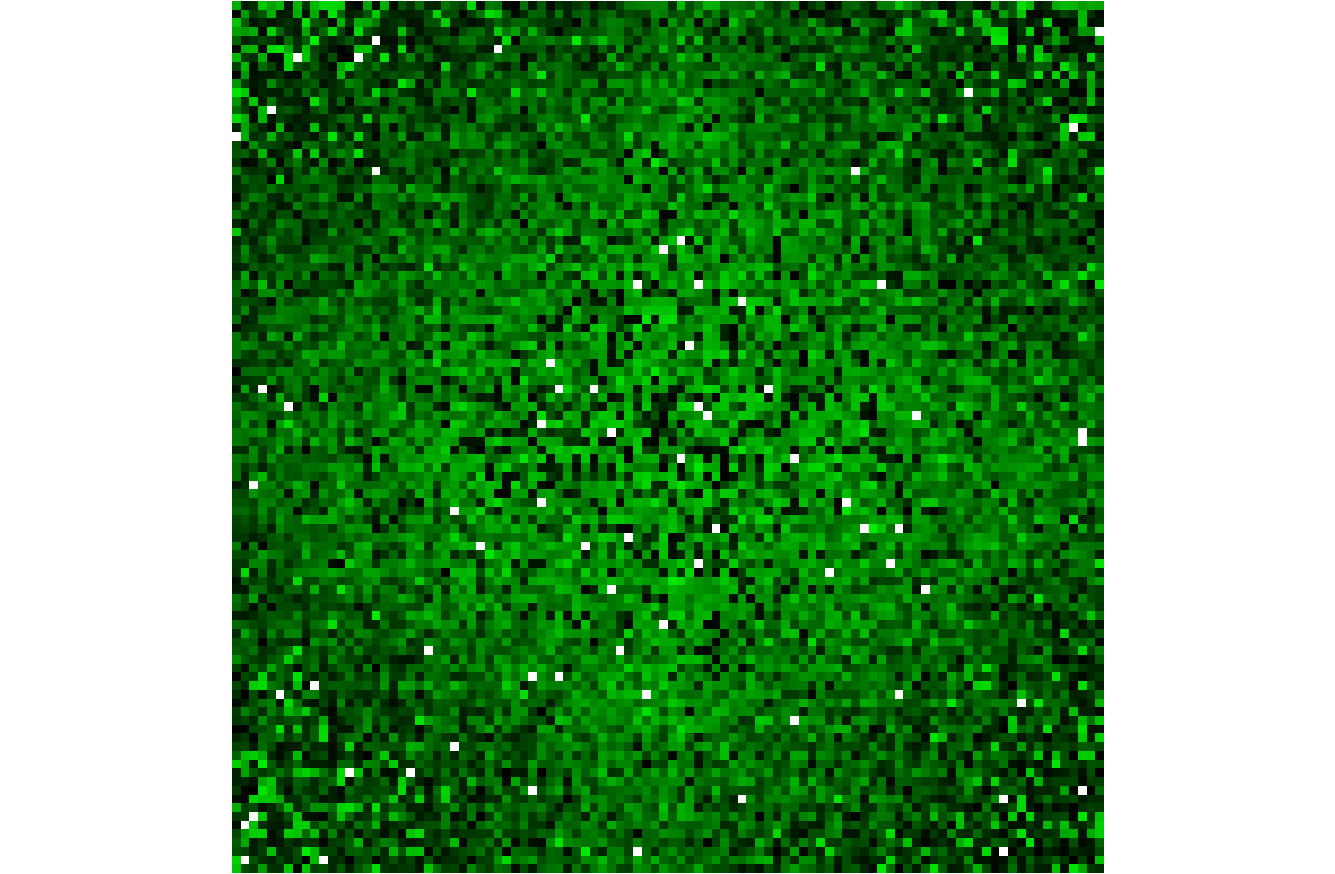
Figure 7.7: The result of the Eden growth algorithm after 400 time steps.
The first couple of time steps look very artificial. Can you remember how to overcome this problem? Check again the chapter on “stochastic cellular automata”!
The trick is done, by introducing a germination probability, e.g. let only 80% of seeds germinate. This is accomplished by comparing with a random draw from hundred: add and 80 > rnd(100) to the if condition in the germination action.
7.2.3 Diffusion-limited aggregation
The diffusion-limited aggregation approach was first described by Witten and Sander (1981). Basically it describes the process, how a crystal grows in a saturated solution:
- Seed a single occupied site
- Each time step: release a ‘random walker’ (an agent that decides which direction to go randomly each time step) on an unoccupied site, anywhere on the grid and let it walk until it senses an occupied site in its neighbourhood. Let the walker stop and occupy that site.
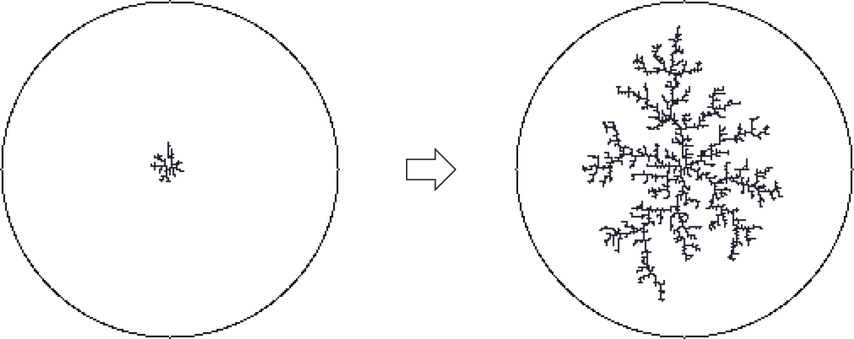
Figure 7.8: Diffusion limited aggregation describes the process, how floating particles attach to a structure.
7.3 Movement
Movement is the third and final category of spatial processes that form the basic ‘building block’ models for spatio-temporal simulation modelling (O’Sullivan and Perry 2013). We will restrict ourselves to explore the movement of zero-dimensional (point-shaped) agents. Movement of objects that are extended in space are more adequately conceptualised as diffusion or spread processes that we discussed in the last slides.
To familiarise ourselves with movement patterns, we start with the simplest type of movement known as ‘random walk’. Then we look into more interesting behaviour that do not move at constant speed, like Lévy flights. Finally, we will explore movement patterns that emerge from purposeful acting agents or from the interactive behaviour between agents.
Movement can act in an underlying grid structure that can easily be coupled with cellular automata. However, moving agents can equally well act on Euclidean space or within a network. The common denominator of most movement models is the use of an agent-based approach.
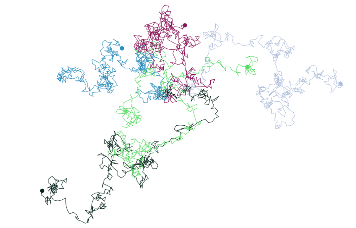
Figure 7.9: Random walk assumes a completely random choice of direction each time step.
In Figure 7.9, you can see the random walk pattern of five agents after 500 time steps. At each time step the direction is defined randomly between 0° and 359° and the step length is one unit.
Although it is fairly unrealistic that a living agent moves completely randomly, it is commonly used in models where the underlying intention of movement does not matter or is not known. Further, the random walk pattern exhibits an interesting behaviour that is very useful to know for model analysis and the detection of spatio-temporal patterns: the root mean square (RMS) of the Euclidean distance that a random walker moves away from its starting point equals the step length (L) times the square root of the walk duration, i.e. the number of steps (t):
\[\sqrt(R^2)=L\sqrt(t)\]
This behaviour can be solved analytically for random walks in lattice structures. Statistically it can also be shown for random walks in Euclidean space. If the step length varies randomly, the general rule that the RMS is proportional to \(\sqrt(t)\) still holds. Even, if we decide to model a walk that has a more persistent direction (a ‘correlated random walk’) by implementing a turn angle instead of a completely random direction, the same pattern emerges on a broader scale.
7.3.1 Lévy flights
Let’s consider a human agent as random walker. This person usually moves in and around his home town, but in rare cases decides to travel over a long distance. Now, the travelled distances do not longer follow a normal distribution, but a distribution with a heavy tail (e.g. Pareto or Cauchy distributions). In this case, the general rule of random walks \(\sqrt(R^2)\sim\sqrt(t)\) does not longer hold. The effectively travelled distance of our human agent is much larger. Moving behaviour like this is called ‘super diffusive’ and it can often be observed in nature, e.g. in the spread of invasive species, the post-glacial recolonisation of trees, or the movement of dollar bills. Even the everyday movement of people can often be described as super-diffusive, as we have just seen.
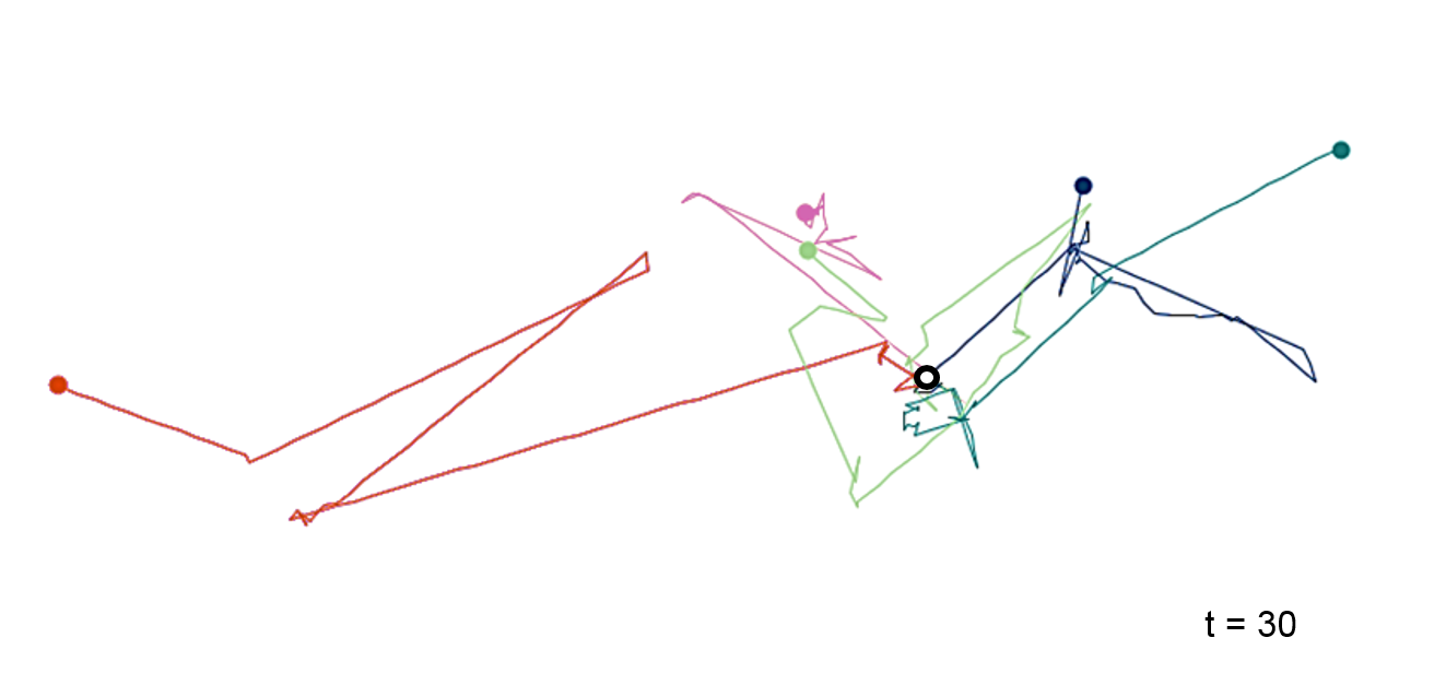
Figure 7.10: Lévy flights are like random walks except for their step length, which follows a distribution with a heavy tail.
However, random walks and its derivatives like persistent walks, or Lévy flights show a pattern that might look like a pattern that we encounter in the real world, but these models do not represent the mechanism of this movement. Or to use the correct terminology: these models are phenomenological, not mechanistic. In the next slides we will discuss more purposeful models of movement.
7.3.2 Moving with a purpose
The representation of agents that move through space following their specific, individual purpose is the core idea of agent-based models. As we have discussed in the respective lesson, agents need to be equipped with certain ‘intelligent’ properties to be able to follow their purpose. An agent needs a goal (e.g. finding food, or a nesting site), a ‘vision’ to be able to see what it is looking for, a decision strategy to prioritise goals in specific situations, and last but not least the ability to move towards the site, where it can satisfy its needs. If the walk was only random, the agent would frequently return to a grid cell where it just has been, which dramatically reduces its success rate to find the required resources. Purposeful movements therefore involves path memory and related walking strategies, such as self-avoiding walk (to avoid just ‘harvested’ sites) or reinforced walk (to revisit sites that have been rich in resources).
Currently active research focusses on the interplay between resources that are heterogeneously distributed across the landscape and adapted (or if learning is involved: adaptive) foraging strategies. For example, Walsh et al. (2010) explored a model on monkeys feeding on seasonally fruiting trees. The intriguing outcome was that overall success rates were higher, if some randomness (‘exploratory urge’) was retained in addition to decision-making based on memory.
In the previous slide we have only considered an agent’s purpose to find non-moving resources. Now, we consider interactive behaviour between moving agents. Concerted moving strategies involve attraction, repulsion or imitation (alignment). From these individual strategies patterns of collective behaviour emerge. One of the most intriguing examples is the flocking behaviour that rapidly emerges from three simple rules:
- If my neighbour is too close: move away
- If my neighbour is too far away: move towards it
- If my neighbour is at a pleasing distance: align to it
This model has successfully been applied to flocking birds, to schooling fish and to herds of land animals. Interestingly, the same model can adequately model the behaviour of human crowds in emergency evacuation situations.
Exercise - Purposeful movement
The “wander” movement command in GAMA covers random walk and correlated random walk. There are two more command to make an agent move: goto target: {point} and move heading: (degrees). Unfortunately, the direction in GAMA is a bit weird: 0° isn’t North, but East.
Let’s start and model an agent to go West. We continue working with the model So, if an agent should go towards West, the heading should be 180°.
    //behaviour: movement
    reflex moveWest {
        do move heading: 180.0 speed: 10 #m/#s bounds:pasture_geom;
    }
Of course, you can define the direction as a moving target. Let the cows head towards one of the other cows:
    //behaviour: movement
    reflex moveToCow0 {
        do move heading: self towards cows[0] speed: 10 #m/#s bounds:pasture_geom;
    }
Alternatively, you could use the goto command for the same movement behaviour. Well, almost the same: can you spot the difference? Also, note that goto doesn’t allow to define bounds for the movement.
    //behaviour: movement
    reflex gotoCow0 {
        do goto target: cows[0].location speed:10 #m/#s ;
    }
If you don’t want your cows to meet at a specific cow, but you want them to cluster together collectively, you can introduce some randomness: at each time step, each cow chooses another cow that it approaches.
    //behaviour: movement
    reflex clusterWithOthers {
        do goto target: cows[int(rnd(4))].location speed:10 #m/#s ;
    }
Social movement
And now, even more sophisticated: you want your cow to goto any other random cow, but only if the closest cow is quite close or far away. Otherwise, you turn away from the closest cow. So that sounds strange. Before checking it out in the simulation: can you predict what will happen?
    //behaviour: movement
    reflex adaptiveMovement {
      if (self distance_to(cows closest_to(self)) < 20) or (self distance_to(cows closest_to(self)) > 50) {
          do goto target: cows[int(rnd(4))].location speed:10 #m/#s ;
      }
      else {
          do move heading: (cows closest_to(self) towards self) speed:10.0;
      }
    }
See explanation.
Congratulations! You have produced a flocking pattern! Did you suspect this would happen? No? Well, exactly that is Emergence: a hard-to-predict, somewhat surprising pattern that arises from adaptive behaviour between agents.